6 Machine learning theory and Support vector machine
Table of contents
- 6.1 Machine learning: Supervised and Unsupervised
- 6.2 SVM: Theory
- 6.3 SVM: Linear SVM
- 6.4 SVM: Non-linear SVM
- 6.5 Classifier evaluation: Confusion matrix and Receiver operating characteristics
- 6.6 Training and Test data: Single dataset hold-out and k-fold cross validation
- 6.7 SVM: Data pre-processing
- 6.8 SVM: Model selection
- 6.9 SVM: Multiclass and Regression
- 6.10 Other supervised learning algorithms: Decision tree, Artificial neural network, Naive Bayesian, and \(k\)-nearest neighbor
- References
The support vector machine (SVM) is a machine learning technique that has been applied in numerous bioinformatics domains successfully in recent years [1]. We used SVM as a machine learning model to achieve the first sub-goal of our research: miRNA target prediction. We built a binary classification model with both linear and non-linear approaches. Binary classification predicts only two class labels, positive/true or negative/false. This chapter describes the theoretical background for SVM, and data preparation and evaluation methods mainly for binary classification, followed by other machine learning algorithms for comparison.
6.1 Machine learning: Supervised and Unsupervised
Machine learning (ML) techniques have two major paradigms, supervised and unsupervised learning. Supervised learning is used for discriminant analysis and regression analysis [2], and it requires a training process. The training data consists of multiple feature vectors and the class labels. The main purpose of the training process is to make a classifier that can predict appropriate class labels from the feature vectors of the test data. The test data consists of the same feature vectors as in the training data, but it has no class labels. Unsupervised learning requires no training process, and it categorizes unlabeled data. The main application of unsupervised learning is clustering. The aim of clustering is to divide the data into groups (clusters) using some measures of similarity [2].
6.2 SVM: Theory
SVM is a state-of-the-art supervised machine learning method introduced by Boser, Guyon, and Vapnik in 1992 [3]. SVM is a linear binary classification method based on the Structural Risk Minimization (SRM) principle [4]. Two essential ideas of SRM are the bound on the generalization performance of a learning machine and the Vapnik Chervonenkis (VC) dimension [5].
The aim of SRM is to find a hypothesis \(h\) that has the guaranteed lowest probability of error \(Err(h)\) from a hypothesis space \(H\) [6]. In other words, SRM finds the best machine learning model, \(\alpha\), that has lowest test error rate, \(R(\alpha)\), where \(R(\alpha)\) is equivalent with \(Err(h)\). The upper bound of the test error can guarantee the performance of a learning machine, and the bound holds with a probability of at least \(1-\eta\) for a given training sample with \(n\) examples [7]:
\[\label{eq_rm_bound} R(\alpha) \leq R_{emp}(\alpha) + \displaystyle \sqrt{\dfrac{d(\log(2n/d)+1)-\log(\eta)}{4}}, \tag{6.1}\]where \(R_{emp}(\alpha)\) is a training error rate, and \(d\) is a VC dimension.
The VC dimension is a measure of capacity for the data point separation by hyperplanes, and this separation is called shattering. A hyperplane in Euclidean space can separate the space into two half spaces, and it is a subset of \(n-1\) dimension for an \(n\)-dimensional space. For example, a straight line is a hyperplane of a two-dimensional Euclidean space, whereas a flat-plane is a hyperplane of a three-dimensional Euclidean space. The VC dimension varies depending on the selection of a machine learning model. For example, the VC dimension of the set of oriented hyperplanes in \(\mathbf{R}^{n}\) is \(n+1\) for a simple linear binary classifier, such as perceptron. Accordingly, Eq. \eqref{eq_rm_bound} reflects a trade-off between the training error, \(R_{emp}(\alpha)\), and the complexity of hypothesis space estimated by the VC-dimension of a learning machine [6].
SVMs solve this trade-off problem by keeping the VC-dimension low through maximizing the margin of boundaries. A SVM can be defined as a linear binary classifier:
\[\label{eq_binary_lnr} f(\mathbf{x}) = sign(\mathbf{w^{T}x} + b) = \left\{ \begin{array}{l l l} +1 & \mathrm{if} & \mathbf{w^{T}x} + b > 0\\ -1 & \mathrm{else} & \\ \end{array} \right. , \tag{6.2}\]where \(w\) is a weight vector and \(b\) is a threshold. The margin of this classifier, \(\delta\), is a length between a boundary hyperplanes, either \(\mathbf{w^{T}x} + b = +1\) or \(\mathbf{w^{T}x} + b = -1\), and the optimal hyperplane, \(\mathbf{w^{T}x} + b = 0\). The margin is calculated as:
\[\label{eq_margin} \delta = \dfrac{1}{||\mathbf{w}||}. \tag{6.3}\]Vapnik proved that the VC dimension \(d\) for such a classifier defined in Eq. \eqref{eq_binary_lnr} is bounded by [4]:
\[\label{eq_vcdimen} d \leq \min \left( \left[ \dfrac{\mathbf{R}^{2}}{\delta^{2}} \right], N \right) + 1, \tag{6.4}\]when this classifier is in an \(N\) dimensional space, and all example vectors, \(\mathbf{x}_{1}, \cdots, \mathbf{x}_{n}\), are inside a ball of diameter \(\mathbf{R}\). It indicates that a SVM classifier keeps the VC-dimension lower by maximizing the margin of the boundaries between two hyperplanes. This is the mathematical background to guarantee that SVM has an upper bound of the test error rate even with very large feature vectors since the number of feature vectors has very small influence on the VC-dimension with SVM.
6.3 SVM: Linear SVM
The aim of SRM is to find an optimal hyperplane than can maximize the right term of Eq. \eqref{eq_rm_bound}. SVM is based on SRM, and its solution is to make a classifier as Eq. \eqref{eq_binary_lnr} with the maximum margin of Eq. \eqref{eq_margin}. In other words, from many boundaries that can separate two classes (Fig. 6.1A), the SVM finds the optimal hyperplane where the margin of the boundary between two hyperplanes, \(\mathbf{w^{T}x} + b = +1\) and \(\mathbf{w^{T}x} + b = -1\) becomes the maximum (Fig. 6.1B). Because it is difficult to solve this maximum margin problem directly, this problem is usually translated into the quadratic optimization problem [6]. Quadratic programming (QP) is a class of optimization algorithms to either minimize or maximize a quadratic function subject to linear constrains. For SVM, finding a solution in the prime form of QP defined in Eq. \eqref{eq_s_prime} is equivalent to finding the optimal hyperplane with the maximum margin. The training data of this SVM are \((\mathbf{x}_i, y_i)\) for \(\forall i\) where \(\mathbf{x}_i\) is a feature vector with \(N\) dimensions as \(\mathbf{x}_i \in \mathbf{R}^{N}\), and \(y_i\) is a class label as \(y_i \in \{-1,+1\}\).
\[\label{eq_s_prime} \begin{array}{l l} \underset{\mathbf{w},b}{\text{minimize}} & \dfrac{1}{2}||\mathbf{w}||^{2} \\ \text{subject to}: &y_{i}(\mathbf{w^{T}x}_{i} + b) \geq 1, \forall i. \end{array} \tag{6.5}\]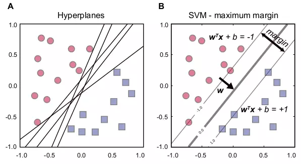
Figure 6.1. SVM hyperplanes and maximum margin.
The figure shows the relationship between hyperplanes and the maximum margin of SVM. Red circle and blue square dots represent data points with negative and positive labels. (A) Many hyperplanes can separate two classes. (B) Three lines represent hyperplanes with the optimal hyperplane in the middle. The margin is a distance between two hyperplanes, \(\mathbf{w^{T}x} + b = +1\) and \(\mathbf{w^{T}x} + b = -1\). \(\mathbf{w}\) is a weight vector.
However, this prime form of QP (Eq. \ref{eq_s_dual}) is still numerically difficult to handle [6], therefore, it can be further transformed into the dual form:
\[\label{eq_s_dual} \begin{array}{l l} \underset{\alpha}{\text{maximize}} & \displaystyle \sum_{i=1}^{n}\alpha_{i} - \dfrac{1}{2} \displaystyle \sum_{i=1}^{n} \displaystyle \sum_{j=1}^{n} y_{i}y_{j}\alpha_{i}\alpha_{j}\mathbf{x}_{i}^{\mathbf{T}}\mathbf{x}_{j}\\ \text{subject to}: & \displaystyle \sum_{i=1}^{n} y_{i}\alpha_{i} = 0, 0 \leq \alpha_{i} \end{array} \tag{6.6}\]Support vectors are vectors such that their corresponding \(\alpha\) values are non-zero in this dual form. SVMs only use these support vectors when classifying the test data. The dot product of \(\mathbf{x}_{i}^{\mathbf{T}}\mathbf{x}_{j}\) can be used for the kernel trick that enables SVMs to solve non-linear problems [8].
In many cases, SVMs can find no hyperplanes that separate two classes, therefore, the slack variables, \(\xi\), are introduced to allow some misclassified data points [6]. The SVM with \(\xi_{i}\) is called a soft-margin SVM [9], and its prime form is:
\[\label{eq_s_prime_c} \begin{array}{l l} \underset{\mathbf{w},b}{\text{minimize}} & \dfrac{1}{2}||\mathbf{w}||^{2} + C \displaystyle \sum_{i=1}^{n} \xi_{i} \\ \text{subject to}: &y_{i}(\mathbf{w^{T}x}_{i} + b) \geq 1 - \xi_{i}, \xi_{i} \geq 0, \forall i, \end{array} \tag{6.7}\]where \(C\) is the cost factor that controls the training error rate. Small \(C\) allows many misclassified points (Fig. 6.2A), whereas large \(C\) allows few misclassified points between the boundaries (Fig. 6.2B).
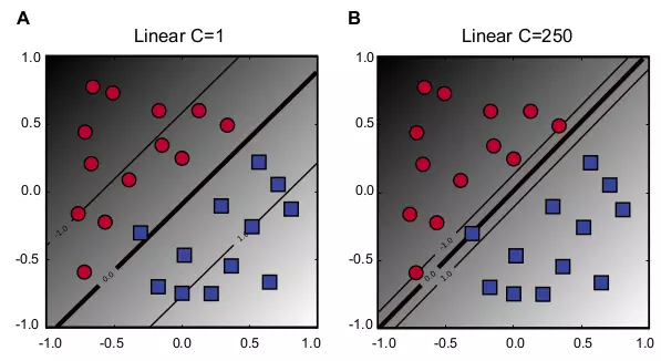
Figure 6.2.Linear kernel with soft margin.
The figure shows two examples of different soft margin constants. Red circle and blue square dots represent data points with negative and positive labels, respectively. Three lines represent hyperplanes with the optimal hyperplane in the middle. The gray scale in the background indicates discriminant values. The darker indicates the smaller in negative values, whereas the lighter indicates the greater in positive values. (A) \(C = 1\). (B) \(C = 250\). In this example, SVM(A), the SVM in panel A, misclassifies one point, whereas SVM(B), the SVM in panel B, classifies all points correctly. However, SVM(A) found a better hyperplane between the overall trends in circle and square classes than SVM(B). SVM(B) has a much smaller margin to the circle class than SVM(A).
6.4 SVM: Non-linear SVM
SVMs can use a kernel function to solve non-linear problems. When the feature vectors are mapped to a high dimensional (\(>d\)) feature space, \(\mathcal{H}\), from the original \(d\)-dimensional feature space, \(\mathbf{R}^{d}\), a non-linear separation in \(\mathbf{R}^{d}\) becomes a linear separation in \(\mathcal{H}\) (Fig. 6.3) [10]. The non-linear mapping function is defined as:
\[\label{eq_hilbert} \Phi: \mathbf{R}^{d} \mapsto \mathcal{H}. \tag{6.8}\]The dot product, \(\mathbf{x}_{i}^{\mathbf{T}}\mathbf{x}_{j}\), in Eq. \eqref{eq_s_dual} can be replaced by a kernel function defined as:
\[\label{eq_kerneltr} K(\mathbf{x}_{i},\mathbf{x}_{j}) = \Phi(\mathbf{x}_{i}^{\mathbf{T}}) \cdot \Phi(\mathbf{x}_{j}). \tag{6.9}\]Two commonly used non-linear kernel functions [2] are Gaussian Radial Basis Function (RBF):
\[\label{eq_rbk} K(\mathbf{x}_{i},\mathbf{x}_{j}) = \exp(-\gamma||\mathbf{x}_{i} - \mathbf{x}_{j}||^{2}),\tag{6.10}\]and Polynomial:
\[\label{eq_poli} K(\mathbf{x}_{i},\mathbf{x}_{j}) = (\mathbf{x}_{i}^{\mathbf{T}} \cdot \mathbf{x}_{j} + 1)^{d}. \tag{6.11}\]These functions are applicable as SVM kernel functions because they can be cast in terms of dot products in Eq. \eqref{eq_kerneltr} [11]. Gaussian RBF has a parameter, gamma \(\gamma\), and Polynomial has a parameter, degree \(d\). These parameters are called kernel parameters, and their optimal values are usually unknown. A common practice to find optimal values for the kernel parameters is to use k-fold cross validation.
Figure 6.3 shows four examples of both Gaussian RBF and Polynomial in two-dimensional space. The gamma parameter in Gaussian RBF represents an RBF width, which is sometimes referred to as \(1/2\sigma^{2}\), and a larger value means a smaller radius. For example, Figure 6.3A has gamma 0.5, and it is less specific and has a larger radius than Figure 6.3B with gamma 4.0. The degree parameter \(d\) in Polynomial is a degree in a polynomial function, as in \(f(x) = a_{d}x^{d} + a_{d-1}x^{d-1} + \cdots + a_{2}x^{2} + a_{1}x + a_{0}\). Figure 6.3C and D show Polynomial kernels with degree 2 and 3, respectively.
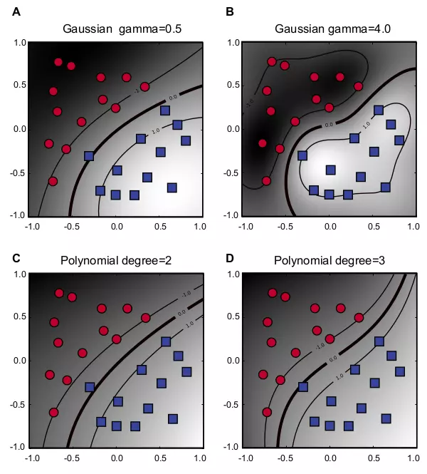
Figure 6.3. Non-linear kernels.
The figure shows four examples of two different non-linear kernel functions in two-dimensional space. Each kernel has two plots with different parameter values. Red circle and blue square dots represent data points with negative and positive labels, respectively. Three lines represent hyperplanes with the optimal hyperplane in the middle. The gray scale in the background indicates discriminant values. The darker indicates the smaller in negative values, whereas the lighter indicates the greater in positive values. The cost factor \(C\) is 10 for all four kernels. (A) Gaussian RBF with \(\gamma = 0.5\). (B) Gaussian RBF with \(\gamma = 4.0\). (C) Polynomial with \(d = 2\). (D) Polynomial with \(d = 3\).
6.5 Classifier evaluation: Confusion matrix and Receiver operating characteristics
A binary classification is a type of classifications that predicts two class labels. To evaluate the performance of a binary classification model, one approach is to use the performance measures derived from the 2 × 2 confusion matrix that shows four possible outcomes with actual and predicted values (Table 6.1)[12]. Another approach is to use Receiver operating characteristics (ROC) [13]. The confusion matrix requires only outcome labels as True or False, whereas ROC requires both outcome labels and discriminant values.
Table 6.1. Confusion matrix.
The table shows four possible outcomes of binary classification.
| Actual value | |||
|---|---|---|---|
| Positive (P) | Negative (N) | ||
| Prediction outcome | Positive | True Positive (TP) | False Positive (FP) |
| Negative | False Negative (FN) | True Negative (TN) |
Standard performance measures that are derived from the confusion matrix are Accuracy (ACC), Error rate (ERR), Sensitivity (SN), Specificity (SP), Positive predictive value (PPV), and Negative predictive value (NPV), and their equations are summarized in Table 6.2. SN, SP, and PPV are also equivalent to True positive rate (TPR), True negative rate (TNR), and Precision (PRC), respectively.
Table 6.2. Performance measures from confusion matrix.
The table shows the term and equation of six performance measures from the confusion matrix.
| Performance measure | Equation |
|---|---|
| Accuracy (ACC) | (TP + TN) / (P + N) |
| Error rate (ERR) | (FP + FN) / (P + N) |
| Sensitivity (SN) | TP / P |
| Specificity (SP) | TN / N |
| Positive predictive value (PPV) | TP / (TP + FP) |
| Negative predictive value (NPV) | TN / (TN + FN) |
A ROC graph is a plot that shows False Positive Rate (FPR) or 1 - SP on the x axis and TPR on the y axis (Fig. 6.4). Many classifiers produce scores or discriminant values that can be used to adjust TPR and FPR. A ROC graph uses these adjusted TPR and FRP to draw curves by changing the threshold values of the scores. A single ROC point is drawn if a classifier has no such adjustment mechanism. A ROC graph contains all information in the confusion metrics, since FN is the complement of TP, and TN is the complement of FP [13]. The area under the ROC curve (AUC) is a performance measure to evaluate the ROC curves. The AUC indicates a perfect prediction and a random prediction when it is 1.0 and 0.5, respectively (Fig. 6.4A). In many cases, the ROC with AUC is a more adequate method to evaluate the classifier performance than single-number measures, such as Accuracy (ACC) [14,15].
It is also important to evaluate the trend of ROC curves. For instance, Figure 6.4B shows two classifiers, Classifier1 and Classifier2, that yield the same AUC scores. Classifier1 is a better classifier despite the same AUC values, because it has a better early retrieval performance, which means it has higher TPR when its SP is also high. The area marked orange in Figure 6.4B is the important region to estimate the early retrieval performance. Two variants of ROC, ROC50 [16] and concentrated ROC (CROC) [17] are especially useful when measuring the early retrieval performance. They are similar to evaluating the ROC curves in the high SP area as in Figure 6.4B, however, the AUC values of ROC50 and CROC can directly indicate the early retrieval performance.
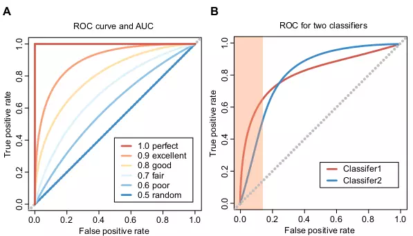
Figure 6.4. ROC curves and AUC scores.
The figures show six ROC curves with corresponding AUC scores and an example ROC plot with two classifiers. (A) The best AUC score is 1, and the worst score is 0. The random guess would yield the AUC score 0.5, and the predictions are opposite to expected when the AUC score is between 0 and 0.5. Six ROC curves have different AUC scores between 0.5 and 1.0 to show different prediction performances. (B) Two classifiers, Classifier1 and Classifier2 have the same AUC scores. The orange area in the left part of the plot indicates the critical area on evaluating ROC curves in terms of the early retrieval performance.
6.6 Training and Test data: Single dataset hold-out and k-fold cross validation
Supervised learning requires a test dataset for performance evaluation. A common problem in machine learning is overfitting, where the model overfits the training data, and it is generalized poorly to unseen data. Therefore, elaborated test procedures are important to maximize the performance and avoid overfitting simultaneously. Two major approaches to separate the test data set from the training data set are single dataset hold-out and k-fold cross validation.
The single dataset hold-out testing is the simplest and most intuitive way to make a test dataset. The sample \(S_{n}\) is divided randomly into two parts, \(S_{l}\) for training and \(S_{k}\) for testing, where the sample size \(n\) is equal to \(l+k\) [6]. \(S_{k}\) is treated as an independent testset, and it should never be used for training. Selecting values of \(l\) and \(k\) is a trade off, because larger \(l\) results in smaller bias of the classifier, and smaller \(k\) increases the variance for the evaluation [6].
Cross validation is the most popular method because the whole dataset is trained and tested. There are several versions of the cross validation approach. Leave-one-out is a good performance estimator in many cases, but it demands very high computational power and it is also sensitive to the data structure. With leave one-out, one data point is removed from the training dataset for testing, and the test procedure continues until each data point is tested. To reduce the computational time, k-fold cross validation is commonly used instead of the leave-one-out approach. In k-fold cross validation, the training set is partitioned into k folds. One fold from the k folds is used as the test dataset, where the remaining dataset with k-1 folds is used for training [6]. 10-fold cross validation with \(k=10\) is widely used for the performance evaluations of classifiers.
Analyzing unbalanced datasets is very common in bioinformatics. For example, some datasets are dominated by negative records with very few positive records, therefore the positive:negative ratio is unbalanced. Unbalanced datasets can present a challenge for any machine learning algorithm to achieve good performance [18,19]. SVM can deal with unbalanced data by assigning different soft-margin constants to each class label [20]. However, it is important to consider this imbalance when making training and test datasets. One approach to solve this imbalance is to use stratification. For example, a stratified k-fold cross validation selects k-fold datasets by sampling data from each subpopulation (stratum), which is a subset of the data with the same class label, independently.
6.7 SVM: Data pre-processing
It is important to process data before training and testing. Two common approaches that may improve the SVM performance are categorical data conversion and scaling.
SVM requires numerical feature vectors, therefore, categorical data need to be transformed. SVM usually achieves better performance when using \(m\) feature vector components to represent an \(m\)-category feature instead of a single component [21]. For example, a feature for a single RNA nucleotide {A,C,G,U} can be represented as (0,0,0,1), (0,0,1,0), (0,1,0,0) and (1,0,0,0).
Scaling is very important for various machine learning algorithms including SVM [22]. Two common ways of scaling are linear scaling [21] and standardizing [20]. With the linear scaling, all vector components are linearly transferred into the same range, for example, [-1, +1] or [0, 1], whereas with the standardizing, they are normalized by their mean and standard deviation.
6.8 SVM: Model selection
The optimization of a classifier is an important phase to maximize the classifier performance. A common practice of model selection with SVM is to evaluate the classifier performance with different kernels and their corresponding parameters. The linear kernel has only one parameter, the soft-margin \(C\), but non-linear kernels tend to have more parameters. The standard method of parameter optimization with two parameters is via grid-search [23]. For example, the Gaussian kernel has two parameters \((C, \gamma)\), and the grid-search is performed by gradually changing the values of both parameters.
6.9 SVM: Multiclass and Regression
In some cases, classifications involve more than two classes. Although some machine learning algorithms are strictly limited to binary classification, there are several SVM approaches that can handle multi-class problems [24]. One example of such SVM multi-class approaches is a one-against-the-rest strategy [6]. This strategy decomposes a multi-class problem into multiple independent binary classifications [24].
A version of SVM for regression is called Support Vector Regression (SVR) [8]. The major difference between SVM and SVR is that the labels are real numbers for SVR rather than categorical data. The optimization problem of SVR is very similar to that of SVM with the prime form as:
\[\label{eq_svr_prime} \begin{array}{l l} \underset{\mathbf{w},b}{\text{minimize}} & \dfrac{1}{2}||\mathbf{w}||^{2} \\ \text{subject to}: & \left\{ \begin{array}{l} \mathbf{w^{T}x}_{i} + b - y_{i} \leq \varepsilon \\ y_{i} - \mathbf{w^{T}x}_{i} - b \leq \varepsilon \\ \end{array} \right. ,\\ \end{array} \tag{6.12}\]where \(\varepsilon\) is used to control the errors. SVR can also be transformed to the dual form and handle soft-margin and kernel functions [8].
6.10 Other supervised learning algorithms: Decision tree, Artificial neural network, Naive Bayesian, and \(k\)-nearest neighbor
Some popular and widely used supervised learning algorithms are Decision tree [25], Artificial Neural Network (ANN) [26], Naive Bayes (NB) [27], and \(k\)-nearest neighbor (\(k\)-NN) [28]. These four algorithms are often used for comparisons with SVM, and they are also introduced as supervised learning algorithms together with SVM [29,10,6,30,2].
Decision tree learning uses a tree-like hierarchical graph with multiple nodes. Three different types of nodes are the root as the first node, internal nodes, and the leaves as terminal nodes. A predicted class label can be obtained when the decision making process reaches a leaf, because each leaf contains a probability distribution over the class labels as the results of training [31]. Some learning algorithms, such as Random Forests [32], can combine multiple decision trees. The Random Forests algorithm makes many different decision trees randomly, and it predicts the class labels by combing the outputs of these decision trees [31].
ANN is a machine learning method that is inspired by the structure and functionalities of biological neural networks in the brain [10,33]. The central nervous system (CNS) in the brain has interconnected networks of neurons that communicate among each other by sending electric pulses through axons, synapses and dendrites. ANN consists of nodes, or “neurons”, that are connected together to form a network that mimics the network in the CNS. The single layered perceptron, which is the simplest form of ANN, is a simple feedforward network [34]. The single layered perceptron can only solve linearly separable problems [33]. The multi-layered perceptron has been developed to solve non-linear problems [26], and it has an input layer, an output layer, and one or more hidden layers in-between. The multi-layered perceptron with the error back-propagation method [35], which is an algorithm that aims at optimizing the weight values by minimizing the errors from the output layer to the hidden layers, enables fairly complex neural networks to solve non-linear problem [26].
The NB classifier is a type of statistical learning algorithm. To obtain the probability model of a class variable \(C\), NB uses Bayes’ theorem:
\[\label{eq_bayes} p(C|X_{1},...,X{n}) = \dfrac{p(C)p(X_{1},...,X{n}|C)}{p(X_{1},...,X{n})}, \tag{6.13}\]and it assumes that all feature variables, \(X_{1},...,X{n}\) are independent. The numerator of Eq. \eqref{eq_bayes} is equivalent to the joint probability model, \(p(C,X_{1},...,X{n})\), which can be expressed as \(p(C)\prod_{i=1}^{n}p(X_{i}|C)\) by the definition of conditionally probability when \(X_{1},...,X{n}\) are independent. Since the denominator of Eq. \eqref{eq_bayes} can be considered as constant, the probability model for a classifier is \(p(C|X_{1},...,X{n}) \propto p(C)\prod_{i=1}^{n}p(X_{i}|C)\). It is easy to calculate the probabilities for the classes from training with this model especially when it is log transformed. The assumption of independence of feature variables is almost always wrong, therefore NB classifiers are usually considered as less accurate [10]. Nonetheless, despite its naive and over simplified assumptions, NB classifiers outperform other sophisticated learning algorithms in some cases [36,29].
\(k\)-NN is an instance-based learning algorithm, which delays the induction or generalization process until the classification phase [10]. When a data point needs to be classified, the distances of the data point from all the training data points are calculated. Subsequently, all the training points are sorted by the calculated distance, and the label that is the most frequent in top \(k\) points is selected as output [2]. \(k\)-NN is very simple, and it can use any type of distance metrics, such as Euclidean, Manhattan, and Minkowsky [10]. However, it is computationally inefficient in some cases especially when the data size is large because \(k\)-NN requires to calculate the lengths at each time of classification.
Both SVM and ANN tend to perform better on data with multi-dimensions and continuous features, but they require large sample size to achieve high accuracy. NB works well with relatively small sample size, but it requires strong (naive) independence assumptions. Decision tree learning performs well with classifying categorical data [10]. It is usually based on a heuristic algorithm, and it fails to find optimal solutions in some cases. \(k\)-NN is very simple to understand and interpret, but it is sensitive to irrelevant features [10].
References
- Pavlidis P, Wapinski I, Noble WS. Support vector machine classification on the web. Bioinformatics 2004;20:586–7. https://doi.org/10.1093/bioinformatics/btg461.
- Tarca AL, Carey VJ, Chen X-wen, Romero R, Drăghici S. Machine learning and its applications to biology. PLoS Computational Biology 2007;3:e116. https://doi.org/10.1371/journal.pcbi.0030116.
- Boser BE, Guyon IM, Vapnik VN. A training algorithm for optimal margin classifiers. Proceedings of the fifth annual workshop on Computational learning theory - COLT ’92, ACM Press; 1992, p. 144–52. https://doi.org/10.1145/130385.130401.
- Vapnik VN. Estimation dependences based on empirical data. New York, USA: Springer-Verlag; 1982.
- Vapnik VN. Statistical learning theory. Wiley, New York; 1998.
- Joachims T. Learning to classify text using support vector machines. Kluwer; 2002.
- Burges CJC. A tutorial on support vector machines for pattern recognition. Data Mining and Knowledge Discovery 1998;2:121–67. https://doi.org/10.1023/a:1009715923555.
- Smola AJ, Schölkopf B. A tutorial on support vector regression. STATISTICS AND COMPUTING; 2003.
- Cortes C, Vapnik V. Support-vector networks. Machine Learning, vol. 20, Springer Science and Business Media LLC; 1995, p. 273–97. https://doi.org/10.1007/bf00994018.
- Kotsiantis SB. Supervised machine learning: a review of classification techniques. Informatica 2007;31:249–68.
- Schölkopf B, Smola AJ, Williamson RC, Bartlett PL. New support vector algorithms. Neural Computation 2000;12:1207–45. https://doi.org/10.1162/089976600300015565.
- Provost FJ, Kohavi R. Glossary of terms. on applied research in machine learning. Machine Learning 1998;30:271–4.
- Swets J. Measuring the accuracy of diagnostic systems. Science 1988;240:1285–93. https://doi.org/10.1126/science.3287615.
- Huang J, Ling CX. Using AUC and accuracy in evaluating learning algorithms. IEEE Transactions on Knowledge and Data Engineering 2005;17:299–310. https://doi.org/10.1109/tkde.2005.50.
- Provost FJ, Fawcett T. Analysis and visualization of classifier performance: comparison under imprecise class and cost distributions. Knowledge Discovery and Data Mining, 1997, p. 43–8.
- Gribskov M, Robinson NL. Use of receiver operating characteristic (ROC) analysis to evaluate sequence matching. Computers & Chemistry 1996;20:25–33. https://doi.org/10.1016/s0097-8485(96)80004-0.
- Swamidass SJ, Azencott C-A, Daily K, Baldi P. A CROC stronger than ROC: measuring, visualizing and optimizing early retrieval. Bioinformatics 2010;26:1348–56. https://doi.org/10.1093/bioinformatics/btq140.
- Provost F. Machine learning from imbalanced data sets 101. Proceedings of the AAAI-2000 Workshop on Imbalanced Data Sets 2000.
- Wu G, Chang EY. Class-boundary alignment for imbalanced dataset learning. In ICML 2003 Workshop on Learning from Imbalanced Data Sets, 2003, p. 49–56.
- Ben-Hur A, Ong CS, Sonnenburg S, Schölkopf B, Rätsch G. Support vector machines and kernels for computational biology. PLoS Computational Biology 2008;4:e1000173. https://doi.org/10.1371/journal.pcbi.1000173.
- Hsu CW, Chang CC, Lin CJ. A practical guide to support vector classification. Taipei, Taiwan: 2003.
- Chang C-C, Lin C-J. LIBSVM: A library for support vector machines. ACM Transactions on Intelligent Systems and Technology 2011;2:1–27. https://doi.org/10.1145/1961189.1961199.
- Ben-Hur A, Weston J. A user’s guide to support vector machines. Methods in Molecular Biology, vol. 609, Humana Press; 2009, p. 223–39. https://doi.org/10.1007/978-1-60327-241-4_13.
- Crammer K, Singer Y. On the algorithmic implementation of multiclass kernel-based vector machines. Journal of Machine Learning Research 2001;2:265–92.
- Murthy SK. Automatic construction of decision trees from data: a multi-disciplinary survey. Data Mining and Knowledge Discovery 1998;2:345–89. https://doi.org/10.1023/a:1009744630224.
- Rumelhart DE, Hinton GE, Williams RJ. Learning internal representations by error propagation. Cambridge, MA, USA: MIT Press; 1986.
- Cestnik B, Kononenko I, Bratko I. ASSISTANT 86: A knowledge-elicitation tool for sophisticated users. In: Bratko I, Lavrac N, editors. European Conference on Machine Learning (ECML), Sigma Press, Wilmslow; 1987, p. 31–45.
- Cover T, Hart P. Nearest neighbor pattern classification. IEEE Transactions on Information Theory 1967;13:21–7. https://doi.org/10.1109/tit.1967.1053964.
- Caruana R, Niculescu-Mizil A. An empirical comparison of supervised learning algorithms. Proceedings of the 23rd international conference on Machine learning - ICML ’06, ACM Press; 2006, p. 161–8. https://doi.org/10.1145/1143844.1143865.
- Yan X, Chao T, Tu K, Zhang Y, Xie L, Gong Y, et al. Improving the prediction of human microRNA target genes by using ensemble algorithm. FEBS Letters 2007;581:1587–93. https://doi.org/10.1016/j.febslet.2007.03.022.
- Kingsford C, Salzberg SL. What are decision trees? Nature Biotechnology 2008;26:1011–3. https://doi.org/10.1038/nbt0908-1011.
- Breiman L. Random forests. Machine Learning, vol. 45, Springer Science and Business Media LLC; 2001, p. 5–32. https://doi.org/10.1023/a:1010933404324.
- Krogh A. What are artificial neural networks? Nature Biotechnology 2008;26:195–7. https://doi.org/10.1038/nbt1386.
- Rosenblatt F. The perceptron: a perceiving and recognizing automaton (Project Para). Cornell Aeronautical Laboratory; 1957.
- Rumelhart DE, Hinton GE, Williams RJ. Learning representations by back-propagating errors. Nature 1986;323:533–6. https://doi.org/10.1038/323533a0.
- Domingos P, Pazzani M. On the optimality of the simple bayesian classifier under zero-one loss. Machine Learning 1997;29:103–30. https://doi.org/10.1023/a:1007413511361.