Supplementary information: A two-step site and mRNA-level model for predicting microRNA targets
Takay Saito and Pål Sætrom
Saito, T and Sætrom, P. A two-step site and mRNA-level model for predicting microRNA targets. BMC Bioinformatics 11, 612 (2010). https://doi.org/10.1186/1471-2105-11-612.
Table of contents
- Supplementary Methods
- Supplementary Results
- Analysis of target site level training data: Selection of seed types influences the coverage of potential target sites
- Prediction of targets with optimal distance sites: Optimal distance is effectively incorporated in our SVM prediction
- Site accessibility and sequence conservation: Explicit usage of site accessibility and sequence conservation do not improve SVM prediction
- Classification vs. Regression: Support vector classification (SVC) performs better than support vector regression (SVR)
- Dataset selection: Different parameters for constructing training or test data do not affect SVM prediction performance
- Supplementary Tables
- Table S1. Target site level features.
- Table S2. Analysis of target site level feature influence.
- Table S3. mRNA level features.
- Table S4. Analysis of mRNA level feature influence.
- Table S5. Benchmarks on the Linsley dataset.
- Table S6. mRNA/siRNA sequences from five microarray experiments.
- Table S7. Parameters used for the Needle software.
- Table S8. Benchmarks on the Selbach dataset.
- Table S9. Benchmarks on the Baek dataset.
- Table S10. Benchmarks on the Linsley dataset – Positive records defined by log ratio -0.1.
- Table S11. Benchmarks on the Linsley dataset – Positive records defined by log ratio -0.3.
- Table S12. Benchmarks on the Selbach dataset – Positive records defined by log ratio -0.1.
- Table S13. Benchmarks on the Selbach dataset – Positive records defined by log ratio -0.3.
- Table S14. Benchmarks on the Baek dataset – Positive records defined by log ratio -0.1.
- Table S15. Benchmarks on the Baek dataset – Positive records defined by log ratio -0.3.
- Supplementary Figures
- Figure S1. 10-fold cross-validation of target site level classifiers trained on three microarray datasets.
- Figure S2. Density plot for the number of potential target sites divided by 3’UTR length.
- Figure S3. Comparison between two SVM trainings with or without explicit addition of negative records.
- Figure S4. 10-fold cross-validation of mRNA level classifiers trained on three microarray datasets.
- Figure S5. Three method-specific benchmarks of 8 different algorithms on the Linsley dataset.
- Figure S6. siRNA benchmarks on the Jackson dataset.
- Figure S7. miRNA benchmarks on the Lim dataset.
- Figure S8. siRNA benchmarks on the Birmingham dataset.
- Figure S9. miRNA benchmarks on the Grimson dataset.
- Figure S10. Targets with optimal distance sites show higher average discriminant value than other three target types.
- Figure S11. Adding site accessibility and sequence conservation features did not affect target prediction accuracy.
- Figure S12. SVC performs better than SVR at both target site and mRNA levels.
- Figure S13. SVM performance is similar between the training set with up-regulated genes and the one without up-regulated genes.
- Figure S14. Two-step SVM retains the performance when trained with proteomics data.
- Figure S15. Benchmarks on the Selbach dataset.
- Figure S16. Benchmarks on the Baek dataset.
- Figure S17. Benchmarks on the Linsley dataset with positive record threshold by log ratio -0.1.
- Figure S18. Benchmarks on the Linley dataset with positive record threshold by log ratio -0.3.
- Figure S19. Benchmarks on the Selbach dataset with positive record threshold by log ratio -0.1.
- Figure S20. Benchmarks on the Selbach dataset with positive record threshold by log ratio -0.3.
- Figure S21. Benchmarks on the Baek dataset with positive record threshold by log ratio -0.1.
- Figure S22. Benchmarks on the Baek dataset with positive record threshold by log ratio -0.3.
- References
Supplementary Methods
Data partition into positive (down-regulated) and negative genes
Down-regulated (positive) genes of GEO datasets were defined as records with p-value < 0.001 and log intensity ratio < -0.3 to obtain strongly down-regulated genes. Down-regulated genes for the Birmingham dataset were obtained directly from the published data [1].
Some microarray records contained different results for the same combination of miRNA/siRNA and mRNA; for example, there were five records of a miRNA on the same mRNA, and four of them were regarded as down-regulated but one of them were unaffected. In this case, all records that belonged to this combination were disregarded to enhance the quality.
Negative records of GEO datasets consisted of both unaffected and up-regulated genes. Unaffected genes were defined as records with p-value > 0.3 and log intensity ratio between -0.3 and 0.3, whereas up-regulated genes were defined as records with p-value < 0.001 and log intensity ratio > 0.3. Negative records for the Birmingham dataset were defined as all RefSeq transcripts except the positive records.
As a final filter, all miRNA:mRNA pairs that had either very high (>1.25) or very low (<-1.5) log intensity values in the control experiments were eliminated to reduce potential noise form extreme expression values.
All the positive records were used in the training dataset, whereas negative records were randomly selected to meet a total record number of 20000, unless otherwise specified. A maximum total record number of 20000 was used due to computational time and memory space constraints.
For the test data, positive records were selected as for the training data, whereas all the remaining records were used as negative records.
For the Linsley dataset [2], down-regulated genes were defined as records with p-value < 0.001 and log intensity ratio < -0.2.
For the Selbach and Baek datasets, down-regulated genes (positive) were defined as records with log ratio values < -0.2, whereas unaffected genes (negative) were defined as log ratio values > 0. The records that do not fit in these criteria were not used in this study.
Data retrieval for benchmarks
Prediction data were downloaded from the Segal Lab site (https://genie.weizmann.ac.il/pubs/mir07/) for PITA All and PITA Top, the TargetScanHuman 5.1 site (http://www.targetscan.org) for TargetScan and TargetScan with conserved genes, the MicroCosm Targets Version 5 site (http://www.ebi.ac.uk/enright-srv/microcosm) for miRanda, the miRDB site (http://mirdb.org) for mirTarget2, and the PicTar WEB INTERFACE site (https://pictar.mdc-berlin.de/) for PicTar. Several methods provide only target site level scores for download, and, in that case, summation methods showed in the web sites or in the original publications were applied to obtain scores for the mRNA level. For siRNA predictions, PITA and TargetScan executable programs were downloaded and used to calculate prediction scores.
Performance evaluation on independent dataset
Six dataset – “ROC with All genes”, “ROC10*n”, “ROC with 7mer + Conservation”, and three method-specific datasets for TargetScan, miRanda, and PicTar – were created for evaluation. The “ROC with All genes” dataset was comprised of all the records from the microarray dataset.
“ROC10*n” was based on the standard ROC50 [3] benchmark. The ROC50 benchmark score is the area under the ROC curve until 50 negatives are found. Consequently, the “ROC10*n” benchmark datasets consisted of all the true positives found in the microarray experiments and the 10*n first negatives found by each method benchmarked.
The “ROC with 7mer + Conservation” dataset was comprised of genes with conserved 8mer or 7mer-m8 or 7mer-A1 sites. Sites were defined as conserved if the average phyloP 44 scores in the seed region were > 0.9.
The three method-specific datasets for TargetScan, miRanda, and PicTar were generated by only using the records from the microarray experiments that had corresponding predictions for each method.
Supplementary Results
Analysis of target site level training data: Selection of seed types influences the coverage of potential target sites
Current methods for miRNA target prediction base their analyses on identifying so-called seed sites in 3’ UTR. The definition of seed types varies from one prediction algorithm to another [4,5,6], however, and this heavily influences the coverage of potential target sites. Lower coverage means that predictions may lack many true positive sites, whereas higher coverage may result in poor accuracy because of too many false positive sites.
Based on four different microarray datasets - Birmingham [1], Jackson [7], Lim [8], and Grimson [5], we identified a set of 823 genes that were down-regulated in response to artificial miRNA or siRNA transfection, or up-regulated in response to miRNA inhibition (see Supplementary Methods). This positive set of genes constituted 0.14% of the 571570 potential miRNA:gene interactions assayed in the microarray experiments. Searching for seed sites among the positive genes identified that 347 and 510 genes contained stringent and all types of seed sites. Thus, basing miRNA target predictions on stringent seeds or all seed types would cover 42% or 62% of the positive genes. The corresponding numbers for the negative set of 570747 genes were 128254 and 31277. Consequently, the predictive accuracy, as measured by the positive predictive value (PPV = True positive predictions / All positive predictions), was almost three times greater for stringent seeds (PPV = 1.1%) than for all seed types (PPV = 0.40%). Even so, this showed that predicting miRNA targets purely based on identifying stringent seed sites would give too many false positive predictions to be viable in practice.
Several approaches have shown that other target-related features besides the seed type and additional data such as miRNA and mRNA expression profiles can improve predictive accuracy [9,10]. We therefore chose to include all seed types to achieve high coverage in the training data and then improve the accuracy through two-step SVM training.
Prediction of targets with optimal distance sites: Optimal distance is effectively incorporated in our SVM prediction
We were interested to see how well the features of optimal distances were incorporated into our algorithm. Our model uses two mRNA features that represent optimal distances: (i) the number of sites that have other neighboring sites within 13-46 nt and (ii) the number of sites that have other neighboring sites within 17-25 nt. Furthermore, one target site level feature, “distance to the next target” could be effective to recognize the targets with optimal distance. However, these features showed little contribution when the influence of both target site and mRNA level features was analyzed (Tables S2 and S4). Therefore, we applied a different approach as to see the difference of prediction power between the target genes with optimal distance and other target genes.
First, we categorized all potential targets into four different target types, which were defined by the number of potential target sites, seed types, and existence of optimal distance sites within the gene’s 3’ UTR. “Single non-stringent” and “Single stringent” were targets that had only one “non-stringent” and “stringent” seed site, whereas “Multiple without optimal distance” and “Multiple with optimal distance” were targets that had multiple sites where none or at least one pair of sites were within . Then, we checked the mRNA level classifier’s distributions of discriminant values for these four target types. The resulting box plots (Fig. S10) show that for each target type, the mRNA-level SVM clearly separates between the positive (down-regulated) and negative (non-down-regulated) targets. Moreover, targets with multiple sites had higher discriminant values than targets with single stringent and single non-stringent sites, and the targets with optimally spaced sites had the highest discriminant values. Thus, site distance contributed positively to the SVM’s predictions.
Site accessibility and sequence conservation: Explicit usage of site accessibility and sequence conservation do not improve SVM prediction
Although target site accessibility is important for both miRNA and siRNA targeting [11,12], it is unclear how useful computational predictions of target site accessibility are for genome-wide miRNA target analyses [13,6]. Similarly, even though many target prediction tools rely on conserved sequences, as these indicate conserved function and targeting, sequences with little or no evidence of conservation can still be functional target sites [14]. Moreover, calculating target site accessibility and conservation features demand much higher computational power and resources than calculating the other features. Therefore, we constructed classifiers without using the site accessibility and sequence conservation features to evaluate their importance in our SVM model.
To evaluate the classifier without of site accessibility and sequence conservation features, we compared the ROC scores of three mRNA level classifiers that used the same mRNA level features, but three different target site classifiers; that is, classifiers (i) without site accessibility and conservational information, (ii) with site accessibility, and (iii) with conservational information. The classifiers were then tested on the independent dataset.
All the results from the 10-fold cross-validation and independent tests showed very little difference among the three classifiers (Fig. S11). Although theoretically sound, the computationally intensive accessibility predictions could therefore, in practice, be eliminated from the SVM classifier. In addition, although many miRNA target sites appear to be well conserved, the small influence of the conservation-related features on SVM performance indicate that many non-conserved miRNA targets exist. This is consistent with the results of the benchmarks of the 8 existing miRNA target prediction methods. Consequently, the proportion of non-conserved miRNA target sites in the set of all potential target sites seems too large to be ignored. Therefore, we opted to train our SVM classifiers without using site accessibility and sequence conservation.
Classification vs. Regression: Support vector classification (SVC) performs better than support vector regression (SVR)
The microarray data used in our experiments measured actual changes in gene expression in response to miRNA or siRNA over-expression. Consequently, even though we treated miRNA target prediction as a classification problem, target prediction could also be solved as a regression problem. To test whether treating target prediction as a regression problem would further improve our predictions, we used the PyML library to train SVR models to fit the log ratio values from the Jackson, Lim, and Grimson microarray experiments. We did not use the Birmingham dataset because pre-processed log ratio values were not available. The SVR models used the same two step approach and the same features as our previous SVC models. The same optimization approach as we used for the SVC models showed that a linear kernel with default parameters gave the best predictions at both the target site and mRNA level. This model selection often resulted in over-fitting or no convergence, however, hence requiring more analysis time than SVC to find an optimal kernel. Moreover, the SVR target site and mRNA level models showed lower prediction performance at the 10-fold cross-validation and independent data set than the SVC models did (Fig. S12). Thus, when the input is based on features derived from the target sequence, classification models are as good or better at predicting miRNA or siRNA target gene expression fold changes as are regression models.
Dataset selection: Different parameters for constructing training or test data do not affect SVM prediction performance
It is important to verify that our SVM approach is still effective when we select different positive (down-regulated) and negative (non-down-regulated) datasets for both training and test because it proves that our SVM approach is not optimized only for a certain parameter criteria of data selection. We generated seven different datasets; one for training and six for independent test sets to further investigate SVM prediction power with different data selection parameters.
Two major steps applied to create datasets in our study were; (i) all microarray datasets were separated into three groups; down-regulated, unaffected and up-regulated, depending of the log ratio values, and (ii) positive data were selected from down-regulated genes, whereas negative records were from both unaffected and up-regulated genes. However, some miRNAs are known to potentially up-regulate genes. The mechanism of this up-regulation is unknown, and the features of up-regulated target sites/genes are possibly quite different from those of miRNAs involved in down-regulation. To check the influence of involving these up-regulated genes in our SVM training sets, we constructed a dataset without up-regulated genes, and trained and tested it on the independent datasets. The 10-fold cross-validation ROC plots for both target site and mRNA level classifiers trained without up-regulated genes (Fig. S13 A, C) were almost identical to those trained with up-regulated genes (Fig. S13 E, G). The prediction power was also retained when the classifiers were tested on the Linsley dataset (Fig. S13 B, D) and compared with those trained with up-regulated genes (Fig. S13 F, H).
Moreover, we generated six independent subsets for one transcriptomics (Linsley) and two proteomics (Selbach and Baek) experiments. Two different positive record datasets defined by log-ratio values <-0.1 and <-0.3 were created for each experiment, resulting in six independent datasets altogether. We performed benchmarks on these datasets and compared with the dataset defined by the log-ratio values <-0.2, which had been used as the default value for all the other benchmarks. The number of positive records detected by all of the eight algorithms in the benchmarks was higher in the log ratio <-0.1 sets; Linsley (Table S10), Selback (Table S12), and Baek (Table S14), and lower in the log ratio <-0.3 sets; Linsley (Table S11), Selback (Table S13), and Baek (Table S15), as expected. The ROC scores from the benchmarks show that SVM outperforms other algorithms in most cases regardless of different parameter criteria of data selection. We also analyzed the ROC curves of the benchmarks to check the trends among the log ratio <-0.2 sets; Linsley (Fig. 5, S5), Selback (Fig. 6, S15) and Baek (Fig.6, S16), the log ratio <-0.1 sets; Linsley (Fig. S17), Selback (Fig. S19) and Baek (Fig. S21), and the log ratio <-0.3 sets; Linsley (Fig. S18), Selback (Fig. S20) and Baek (Fig. S22). All ROC curves showed very similar trends among different positive record sets. More importantly, our SVM approach retained its prediction power even when it was tested on the log ratio <-0.3 and <-0.1 sets.
These results indicate that our SVM prediction power is not affected when trained with or without up-regulated genes, or tested on strongly down-regulated pairs (log ratio <-0.3) as well as moderately down-regulated pairs (log ratio <-0.1).
Supplementary Tables
Table S1. Target site level features.
| Feature | Vector sizea | Siteb | Consvc | Incld | |
|---|---|---|---|---|---|
| 1 | Seed Type | 9 | ○ | ||
| 2 | Similarity (1-20 nt) | 1 | ○ | ||
| 3 | Similarity in the 5' portion (1-9 nt) | 1 | ○ | ||
| 4 | Similarity in the 3' portion (>10 nt) | 1 | ○ | ||
| 5 | Similarity in the 3' portion (position 13,14,15,16 ) | 1 | ○ | ||
| 6 | A:U rich context in the 30nt upstream | 30 | ○ | ||
| 7 | A:U rich context in the 30nt downstream | 30 | ○ | ||
| 8 | Relative site position (position / 3’ UTR length) | 1 | ○ | ||
| 9 | Distance to the next-nearest-neighbor site | 1 | ○ | ||
| 10 | Site accessibility: dGduplex | 1 | ○ | ||
| 11 | Site accessibility: dGopen | 1 | ○ | ||
| 12 | Site accessibility: ddG | 1 | ○ | ||
| 13 | Site accessibility with 3/15 flank: dGopen | 1 | ○ | ||
| 14 | Site accessibility with 3/15 flank: ddG | 1 | ○ | ||
| 15 | 20nt site matches (Match:1, AU:0.4, None-match:0) | 20 | ○ | ||
| 16 | Pos 1 nucleotide of the target site (A:1, UCG:0) | 1 | ○ | ||
| 17 | multiz17way score for the seed site | 1 | ○ | ||
| 18 | multiz17way score for the target site | 1 | ○ | ||
| 19 | PhastCons44way scores for the target site | 1 | ○ | ||
| 20 | PhastCons44wayMammal scores for the target site | 1 | ○ | ||
| 21 | PhastCons44wayPrimate scores for the target site | 1 | ○ | ||
| 22 | PhyloP44ways scores for the seed site | 8 | ○ | ||
| 23 | PhyloP44waysMammal scores for the seed site | 8 | ○ | ||
| 24 | PhyloP44waysPrimate scores for the seed site | 8 | ○ |
aVector size used in SVM training. bSite accessibility features. ○: Yes, blank: No. cSequence conservation features. ○: Yes, Blank: No. dFeatures included in the final version of our classifier. ○: included features, blank: features excluded during optimization steps.
Table S2. Analysis of target site level feature influence.
| Rank | ROC | ROC diffa | Removed feature |
|---|---|---|---|
| 1 | 0.6734 | 0.0317 | Seed Type |
| 2 | 0.6958 | 0.0093 | 20nt site matches (Match:1, AU:0.4, None-match:0) |
| 3 | 0.6998 | 0.0053 | A:U rich context in the 30nt upstream |
| 4 | 0.7047 | 0.0004 | PhastCons44wayMammal scores for the target site |
| 5 | 0.7047 | 0.0003 | Similarity in the 3' portion (>10 nt) |
| 6 | 0.7048 | 0.0002 | Relative site position (position / 3’UTR length) |
| 7 | 0.7049 | 0.0001 | Similarity in the 5' portion (1-9 nt) |
| 8 | 0.7050 | 0.0000 | Site accessibility: dGopen |
| 9 | 0.7050 | 0.0000 | Distance to the next-nearest-neighbor site |
| 10 | 0.7050 | 0.0000 | Site accessibility: dGduplex |
| 11 | 0.7050 | 0.0000 | Site accessibility: ddG |
| 12 | 0.7050 | 0.0000 | Site accessibility with 3/15 flank: dGopen |
| 13 | 0.7050 | 0.0000 | Site accessibility with 3/15 flank: ddG |
| 14 | 0.7051 | -0.0001 | Similarity in the 3' portion (position 13,14,15,16 ) |
| 15 | 0.7053 | -0.0002 | PhyloP44ways scores for the seed site |
| 16 | 0.7054 | -0.0003 | Similarity (1-20 nt) |
| 17 | 0.7054 | -0.0004 | multiz17way score for the seed site |
| 18 | 0.7056 | -0.0006 | Pos 1 nucleotide of the target site (A:1, UCG:0) |
| 19 | 0.7057 | -0.0006 | A:U rich context in the 30nt downstream |
| 20 | 0.7059 | -0.0008 | multiz17way score for the target site |
| 21 | 0.7060 | -0.0009 | PhastCons44wayPrimate scores for the target site |
| 22 | 0.7064 | -0.0014 | PhyloP44waysMammal scores for the seed site |
| 23 | 0.7068 | -0.0017 | PhastCons44way scores for the target site |
| 24 | 0.7081 | -0.0030 | PhyloP44waysPrimate scores for the seed site |
aROC diff shows the difference of ROC scores between the classifier trained with all the features (0.7050) and classifiers trained with one feature removed.
Table S3. mRNA level features.
| Feature | Vector sizea | Inclb | |
|---|---|---|---|
| 1 | 3'UTR Length | 1 | ○ |
| 2 | Number of target sites | 1 | ○ |
| 3 | Total discriminant value / 3’ UTR length | 1 | ○ |
| 4 | Number of 8mer sites | 1 | ○ |
| 5 | Number of 7mer-m8 sites | 1 | ○ |
| 6 | Number of 7mer-A1 sites | 1 | ○ |
| 7 | Number of 6mer sites | 1 | ○ |
| 8 | Number of GUM sites | 1 | ○ |
| 9 | Number of GUT sites | 1 | ○ |
| 10 | Number of LP sites | 1 | ○ |
| 11 | Number of BT sites | 1 | ○ |
| 12 | Number of BM sites | 1 | ○ |
| 13 | Distribution bins of discriminant values | 16 | ○ |
| 14 | Site counts within optimal distance 14-46 nt | 1 | ○ |
| 15 | Site counts within optimal distance 17-25 nt | 1 | ○ |
| 16 | Site number flags (1 or 2-7 or >8) | 3 | ○ |
| 17 | Total discriminant value | 1 | ○ |
aVector size used in SVM training. bFeatures included in the final version of our classifier. ○: included features, blank: features excluded during optimization steps.
Table S4. Analysis of mRNA level feature influence.
| Rank | ROC | ROC diffa | Removed feature |
|---|---|---|---|
| 1 | 0.7565 | 0.0432 | Distribution bins of discriminant values |
| 2 | 0.7904 | 0.0093 | Number of GUM sites |
| 3 | 0.7971 | 0.0026 | Site number flags (1 or 2-7 or >8) |
| 4 | 0.7978 | 0.0019 | Total discriminant value / 3' UTR length |
| 5 | 0.7981 | 0.0016 | Number of 7mer-m8 sites |
| 6 | 0.7984 | 0.0013 | Site counts within optimal distance 17-25 nt |
| 7 | 0.7986 | 0.0011 | Number of BT sites |
| 8 | 0.7994 | 0.0003 | Number of 6mer sites |
| 9 | 0.7995 | 0.0002 | Number of 7mer-A1 sites |
| 10 | 0.7996 | 0.0001 | Total discriminant value |
| 11 | 0.7996 | 0.0001 | 3' UTR Length |
| 12 | 0.7996 | 0.0001 | Number of GUT sites |
| 13 | 0.7997 | 0.0000 | Number of BM sites |
| 14 | 0.7997 | 0.0000 | Number of 8mer sites |
| 15 | 0.7999 | -0.0002 | Number of LP sites |
| 16 | 0.8003 | -0.0006 | Site counts within optimal distance 14-46 nt |
| 17 | 0.8009 | -0.0012 | Number of target sites |
aROC diff shows the difference of ROC scores between the classifier trained with all the features (0.7997) and classifiers trained with one feature removed.
Table S5. Benchmarks on the Linsley dataset.
| Benchmark | Method | # of targetsa | ROCb | |
|---|---|---|---|---|
| Positive | Negative | |||
| All genes | All | 667 | 158374 | |
| SVM | 564 | 69037 | 0.81 | |
| PITA | 539 | 55953 | 0.76 | |
| TargetScan | 400 | 21228 | 0.75 | |
| miRanda | 93 | 6641 | 0.55 | |
| PITA_top | 147 | 4867 | 0.6 | |
| TargetScan_consv | 174 | 5634 | 0.61 | |
| mirTarget2 | 191 | 3386 | 0.63 | |
| PicTar | 124 | 3826 | 0.58 | |
| ROC10*n | All | 667 | 90 | |
| SVM | 16 | 90 | 0.0168 | |
| PITA | 1 | 90 | 0.0058 | |
| TargetScan | 13 | 90 | 0.0267 | |
| miRanda | 11 | 90 | 0.0144 | |
| PITA_top | 2 | 90 | 0.0076 | |
| TargetScan_consv | 14 | 90 | 0.0209 | |
| mirTarget2 | 19 | 90 | 0.0235 | |
| PicTar | 17 | 90 | 0.0151 | |
| 7mer + Conservation | All | 353 | 15823 | |
| SVM | 339 | 12731 | 0.73 | |
| PITA | 339 | 13230 | 0.61 | |
| TargetScan | 310 | 10715 | 0.69 | |
| miRanda | 93 | 6641 | 0.43 | |
| PITA_top | 147 | 4867 | 0.57 | |
| TargetScan_consv | 174 | 5634 | 0.59 | |
| mirTarget2 | 191 | 3386 | 0.67 | |
| PicTar | 124 | 3826 | 0.57 | |
| TargetScan | All | 174 | 5658 | |
| SVM | 168 | 5022 | 0.67 | |
| PITA | 174 | 5440 | 0.56 | |
| TargetScan | 174 | 5634 | 0.65 | |
| miRanda | 36 | 827 | 0.53 | |
| PITA_top | 119 | 3527 | 0.56 | |
| TargetScan_consv | 174 | 5634 | 0.65 | |
| mirTarget2 | 109 | 1926 | 0.66 | |
| PicTar | 87 | 2418 | 0.57 | |
| miRanda | All | 93 | 6641 | |
| SVM | 89 | 4301 | 0.82 | |
| PITA | 88 | 4942 | 0.69 | |
| TargetScan | 82 | 3072 | 0.8 | |
| miRanda | 93 | 6641 | 0.61 | |
| PITA_top | 31 | 801 | 0.61 | |
| TargetScan_consv | 36 | 819 | 0.64 | |
| mirTarget2 | 41 | 602 | 0.67 | |
| PicTar | 25 | 554 | 0.6 | |
| PicTar | All | 124 | 3826 | |
| SVM | 119 | 3683 | 0.69 | |
| PITA | 122 | 3420 | 0.61 | |
| TargetScan | 105 | 3003 | 0.63 | |
| miRanda | 25 | 554 | 0.53 | |
| PITA_top | 92 | 2152 | 0.63 | |
| TargetScan_consv | 87 | 2406 | 0.61 | |
| mirTarget2 | 77 | 1408 | 0.67 | |
| PicTar | 124 | 3826 | 0.65 |
aPositive and Negative show the total number of positive (down-regulated) and negative (unaffected) genes present within the six benchmarks (Method “All”) and among the predictions of each method on the six benchmarks. bROC is the method’s ROC score on the specific benchmark.
Table S6. mRNA/siRNA sequences from five microarray experiments.
| Accession | miRNA/siRNA name | Sequence | Strand | miRNA/siRNA |
|---|---|---|---|---|
| GSE5814 | MAPK14-pos1 mismatch | CCUACAGAGAACUGCGGUA | sense | siRNA |
| GSE5814 | MAPK14-pos2 mismatch | CCUACAGAGAACUGCGGAU | sense | siRNA |
| GSE5814 | MAPK14-pos8 mismatch | CCUACAGAGAAAUGCGGUU | sense | siRNA |
| GSE5814 | MAPK14-pos7 mismatch | CCUACAGAGAACGGCGGUU | sense | siRNA |
| GSE5814 | MAPK14-pos6 mismatch | CCUACAGAGAACUACGGUU | sense | siRNA |
| GSE5814 | MAPK14-pos4 mismatch | CCUACAGAGAACUGCAGUU | sense | siRNA |
| GSE5814 | MAPK14-pos3 mismatch | CCUACAGAGAACUGCGAUU | sense | siRNA |
| GSE5814 | MAPK14-193a | CCUACAGAGAACUGCGGUU | sense | siRNA |
| GSE5814 | PLK1 1319 | CACGCCTCATCCTCTACAA | sense | siRNA |
| GSE5814 | PLK1 772 | GAGACCTACCTCCGGATCA | sense | siRNA |
| GSE5814 | MAPK14-pos5 mismatch | CCUACAGAGAACUGAGGUU | sense | siRNA |
| GSE5814 | PIK3CB-6338 | GUGACAACAUCAUGGUCAA | sense | siRNA |
| GSE5814 | PIK3CB-6340 | CUCCUAAUAUGAAUCCUAU | sense | siRNA |
| GSE2075 | miR-1 | UGGAAUGUAAAGAAGUAUGUAA | antisense | miRNA |
| GSE2075 | miR-124 | UAAGGCACGCGGUGAAUGCCA | antisense | miRNA |
| GSE2075 | miR-124mut5-6 | UAAGCGACGCGGUGAAUGCCA | antisense | siRNA |
| GSE2075 | miR-373 | GAAGUGCUUCGAUUUUGGGGUGU | antisense | miRNA |
| GSE6838 | hsa-miR-16 | UAGCAGCACGUAAAUAUUGGCG | antisense | miRNA |
| GSE6838 | hsa-miR-15a | UAGCAGCACAUAAUGGUUUGUG | antisense | miRNA |
| GSE6838 | hsa_miR_106b | UAAAGUGCUGACAGUGCAGAU | antisense | miRNA |
| GSE6838 | hsa_miR_103 | AGCAGCAUUGUACAGGGCUAUGA | antisense | miRNA |
| GSE6838 | hsa-miR-192 | CUGACCUAUGAAUUGACAGCC | antisense | miRNA |
| GSE6838 | hsa-miR-215 | AUGACCUAUGAAUUGACAGAC | antisense | miRNA |
| GSE6838 | hsa-miR-17-5p | CAAAGUGCUUACAGUGCAGGUAGU | antisense | miRNA |
| GSE6838 | hsa-miR-20 | UAAAGUGCUUAUAGUGCAGGUA | antisense | miRNA |
| GSE6838 | hsa-let-7c | UGAGGUAGUAGGUUGUAUGGUU | antisense | miRNA |
| GSE8501 | hsa-miR-7 | UGGAAGACUAGUGAUUUUGUUG | antisense | miRNA |
| GSE8501 | hsa-miR-9 | UCUUUGGUUAUCUAGCUGUAUGA | antisense | miRNA |
| GSE8501 | hsa-miR-122a | UGGAGUGUGACAAUGGUGUUUGU | antisense | miRNA |
| GSE8501 | hsa-miR-128a | UCACAGUGAACCGGUCUCUUUU | antisense | miRNA |
| GSE8501 | hsa-miR-132 | UAACAGUCUACAGCCAUGGUCG | antisense | miRNA |
| GSE8501 | hsa-miR-133a | UUGGUCCCCUUCAACCAGCUGU | antisense | miRNA |
| GSE8501 | hsa-miR-142-3p | UGUAGUGUUUCCUACUUUAUGGA | antisense | miRNA |
| GSE8501 | hsa-miR-148a | UCAGUGCACUACAGAACUUUGU | antisense | miRNA |
| GSE8501 | hsa-miR-181a | AACAUUCAACGCUGUCGGUGAGU | antisense | miRNA |
| E-MEXP-668 | C52 | CAGGGCGGAGACTTCACCA | sense | siRNA |
| E-MEXP-668 | G4 | TGGTTTACATGTTCCAATA | sense | siRNA |
| E-MEXP-668 | C4 | GGAAAGACTGTTCCAAAAA | sense | siRNA |
| E-MEXP-668 | G41 | GTATGACAACAGCCTCAAG | sense | siRNA |
| E-MEXP-668 | M3 | GAGGTTCTCTGGATCAAGT | sense | siRNA |
| E-MEXP-668 | M1 | GCACATGGATGGAGGTTCT | sense | siRNA |
| E-MEXP-668 | M2 | GCAGAGAGAGCAGATTTGA | sense | siRNA |
| E-MEXP-668 | C14 | GGCCTTAGCTACAGGAGAG | sense | siRNA |
| E-MEXP-668 | C1 | GAAAGAGCATCTACGGTGA | sense | siRNA |
| E-MEXP-668 | C2 | GAAAGGATTTGGCTACAAA | sense | siRNA |
| E-MEXP-668 | C3 | ACAGCAAATTCCATCGTGT | sense | siRNA |
| E-MEXP-668 | M4 | GAGCAGATTTGAAGCAACT | sense | siRNA |
| Selbach | hsa-miR-30a | UGUAAACAUCCUCGACUGGAAG | antisense | miRNA |
| Selbach | hsa-miR-16 | UAGCAGCACGUAAAUAUUGGCG | antisense | miRNA |
| Selbach | hsa-miR-155 | UUAAUGCUAAUCGUGAUAGGGGU | antisense | miRNA |
| Selbach | hsa-miR-1 | UGGAAUGUAAAGAAGUAUGUAU | antisense | miRNA |
| Selbach | hsa-let-7b | UGAGGUAGUAGGUUGUGUGGUU | antisense | miRNA |
| Baek | hsa-mir-181a | AACAUUCAACGCUGUCGGUGAGU | antisense | miRNA |
| Baek | hsa-mir-124 | UAAGGCACGCGGUGAAUGCC | antisense | miRNA |
| Baek | hsa-mir-1 | UGGAAUGUAAAGAAGUAUGUAU | antisense | miRNA |
Jackson (GSE5814), Lim (GSE2075), Grimson (GSE8501), and Birmingham (E-MEXP-668) were used for training, and Linsley (GSE6838) was used for the independent test. Two datasets, Selbach and Baek, from mass spectrometry experiments were used as both training datasets (for the proteomics-based classifiers) and independent test sets (for the mRNA-based classifiers).
aMAPK14-193 has three different sample groups; (i) GSM133702 and GSM134468, (ii) GSM134488, and (iii) GSM134491. We assigned three different unique IDs to these groups, therefore they were treated as different sequences internally in our model.
Table S7. Parameters used for the Needle software.
| Parameter | Value | ||||
|---|---|---|---|---|---|
| Gap open (‑gapopen) | 10.0 | ||||
| Gap extend (‑gapextend) | 7.0 | ||||
| Scoring matrix (‑datafile) | A | U | G | C | |
| A | -3 | 5 | -3 | -3 | |
| U | 5 | -3 | 2 | -3 | |
| G | -3 | 2 | -3 | 5 | |
| C | -3 | -3 | 5 | -3 |
The scoring matrix was generated based on the matrix used in the miRanda algorithm [15].
Table S8. Benchmarks on the Selbach dataset.
| Benchmark | Method | # of targetsa | ROCb | |
|---|---|---|---|---|
| Positive | Negative | |||
| All genes | All | 2311 | 12890 | |
| SVM | 1493 | 5936 | 0.64 | |
| PITA | 1230 | 4276 | 0.61 | |
| TargetScan | 688 | 1220 | 0.61 | |
| miRanda | 183 | 493 | 0.52 | |
| PITA_top | 266 | 274 | 0.55 | |
| TargetScan_consv | 305 | 309 | 0.55 | |
| mirTarget2 | 205 | 155 | 0.54 | |
| PicTar | 185 | 175 | 0.53 | |
| ROC10*n | All | 2311 | 50 | |
| SVM | 95 | 50 | 0.0253 | |
| PITA | 17 | 50 | 0.0042 | |
| TargetScan | 84 | 50 | 0.0212 | |
| miRanda | 28 | 50 | 0.0079 | |
| PITA_top | 57 | 50 | 0.0138 | |
| TargetScan_consv | 82 | 50 | 0.0213 | |
| mirTarget2 | 83 | 50 | 0.0231 | |
| PicTar | 81 | 50 | 0.021 | |
| 7mer + Conservation | All | 576 | 1005 | |
| SVM | 560 | 800 | 0.71 | |
| PITA | 554 | 835 | 0.61 | |
| TargetScan | 495 | 616 | 0.69 | |
| miRanda | 183 | 493 | 0.42 | |
| PITA_top | 266 | 274 | 0.6 | |
| TargetScan_consv | 305 | 309 | 0.63 | |
| mirTarget2 | 205 | 155 | 0.6 | |
| PicTar | 185 | 175 | 0.58 | |
| TargetScan | All | 306 | 313 | |
| SVM | 305 | 298 | 0.63 | |
| PITA | 302 | 310 | 0.52 | |
| TargetScan | 305 | 309 | 0.63 | |
| miRanda | 76 | 41 | 0.56 | |
| PITA_top | 187 | 172 | 0.55 | |
| TargetScan_consv | 305 | 309 | 0.63 | |
| mirTarget2 | 133 | 84 | 0.59 | |
| PicTar | 139 | 125 | 0.55 | |
| miRanda | All | 183 | 493 | |
| SVM | 169 | 305 | 0.76 | |
| PITA | 166 | 328 | 0.66 | |
| TargetScan | 131 | 152 | 0.74 | |
| miRanda | 183 | 493 | 0.54 | |
| PITA_top | 68 | 41 | 0.64 | |
| TargetScan_consv | 76 | 39 | 0.67 | |
| mirTarget2 | 58 | 28 | 0.63 | |
| PicTar | 54 | 29 | 0.62 | |
| PicTar | All | 185 | 175 | |
| SVM | 185 | 172 | 0.61 | |
| PITA | 184 | 172 | 0.54 | |
| TargetScan | 168 | 163 | 0.62 | |
| miRanda | 54 | 29 | 0.56 | |
| PITA_top | 126 | 94 | 0.58 | |
| TargetScan_consv | 139 | 124 | 0.6 | |
| mirTarget2 | 86 | 47 | 0.6 | |
| PicTar | 185 | 175 | 0.62 |
aPositive and Negative show the total number of positive (down-regulated) and negative (unaffected) genes present within the six benchmarks (Method “All”) and among the predictions of each method on the six benchmarks. bROC is the method’s ROC score on the specific benchmark.
Table S9. Benchmarks on the Baek dataset.
| Benchmark | Method | # of targetsa | ROCb | |
|---|---|---|---|---|
| Positive | Negative | |||
| All genes | All | 1301 | 4257 | |
| SVM | 725 | 2005 | 0.56 | |
| PITA | 605 | 1481 | 0.56 | |
| TargetScan | 319 | 557 | 0.56 | |
| miRanda | 81 | 216 | 0.51 | |
| PITA_top | 103 | 143 | 0.52 | |
| TargetScan_consv | 142 | 172 | 0.53 | |
| mirTarget2 | 70 | 92 | 0.52 | |
| PicTar | 73 | 102 | 0.52 | |
| ROC10*n | All | 1301 | 30 | |
| SVM | 39 | 30 | 0.0193 | |
| PITA | 15 | 30 | 0.0046 | |
| TargetScan | 28 | 30 | 0.0157 | |
| miRanda | 17 | 30 | 0.0081 | |
| PITA_top | 31 | 30 | 0.0148 | |
| TargetScan_consv | 32 | 30 | 0.0174 | |
| mirTarget2 | 23 | 30 | 0.0086 | |
| PicTar | 29 | 30 | 0.0131 | |
| 7mer + Conservation | All | 258 | 486 | |
| SVM | 235 | 407 | 0.59 | |
| PITA | 234 | 389 | 0.6 | |
| TargetScan | 217 | 322 | 0.62 | |
| miRanda | 81 | 216 | 0.44 | |
| PITA_top | 103 | 143 | 0.56 | |
| TargetScan_consv | 142 | 172 | 0.61 | |
| mirTarget2 | 70 | 92 | 0.54 | |
| PicTar | 73 | 102 | 0.54 | |
| TargetScan | All | 142 | 176 | |
| SVM | 136 | 169 | 0.57 | |
| PITA | 135 | 164 | 0.57 | |
| TargetScan | 142 | 172 | 0.57 | |
| miRanda | 28 | 32 | 0.5 | |
| PITA_top | 86 | 98 | 0.56 | |
| TargetScan_consv | 142 | 172 | 0.57 | |
| mirTarget2 | 48 | 54 | 0.52 | |
| PicTar | 51 | 58 | 0.52 | |
| miRanda | All | 81 | 216 | |
| SVM | 65 | 144 | 0.64 | |
| PITA | 70 | 142 | 0.62 | |
| TargetScan | 51 | 83 | 0.62 | |
| miRanda | 81 | 216 | 0.5 | |
| PITA_top | 21 | 32 | 0.56 | |
| TargetScan_consv | 28 | 31 | 0.59 | |
| mirTarget2 | 19 | 25 | 0.55 | |
| PicTar | 16 | 16 | 0.57 | |
| PicTar | All | 73 | 102 | |
| SVM | 73 | 100 | 0.54 | |
| PITA | 71 | 91 | 0.62 | |
| TargetScan | 65 | 85 | 0.63 | |
| miRanda | 16 | 16 | 0.53 | |
| PITA_top | 42 | 48 | 0.6 | |
| TargetScan_consv | 51 | 57 | 0.63 | |
| mirTarget2 | 27 | 26 | 0.56 | |
| PicTar | 73 | 102 | 0.59 |
aPositive and Negative show the total number of positive (down-regulated) and negative (unaffected) genes present within the six benchmarks (Method “All”) and among the predictions of each method on the six benchmarks. bROC is the method’s ROC score on the specific benchmark.
Table S10. Benchmarks on the Linsley dataset – Positive records defined by log ratio -0.1.
| Benchmark | Method | # of targetsa | ROCb | |
|---|---|---|---|---|
| Positive | Negative | |||
| All genes | All | 851 | 158190 | |
| SVM | 692 | 68909 | 0.79 | |
| PITA | 655 | 55837 | 0.74 | |
| TargetScan | 474 | 21154 | 0.73 | |
| miRanda | 110 | 6624 | 0.54 | |
| PITA_top | 180 | 4834 | 0.59 | |
| TargetScan_consv | 221 | 5587 | 0.61 | |
| mirTarget2 | 231 | 3346 | 0.62 | |
| PicTar | 159 | 3791 | 0.58 | |
| ROC10*n | All | 851 | 90 | |
| SVM | 20 | 90 | 0.0133 | |
| PITA | 1 | 90 | 0.0014 | |
| TargetScan | 13 | 90 | 0.0147 | |
| miRanda | 13 | 90 | 0.0093 | |
| PITA_top | 4 | 90 | 0.0039 | |
| TargetScan_consv | 14 | 90 | 0.0142 | |
| mirTarget2 | 22 | 90 | 0.0186 | |
| PicTar | 19 | 90 | 0.0106 | |
| 7mer + Conservation | All | 425 | 15751 | |
| SVM | 409 | 12661 | 0.73 | |
| PITA | 404 | 13165 | 0.60 | |
| TargetScan | 368 | 10657 | 0.70 | |
| miRanda | 110 | 6624 | 0.43 | |
| PITA_top | 180 | 4834 | 0.57 | |
| TargetScan_consv | 221 | 5587 | 0.61 | |
| mirTarget2 | 231 | 3346 | 0.67 | |
| PicTar | 159 | 3791 | 0.58 | |
| TargetScan | All | 221 | 5611 | |
| SVM | 215 | 4975 | 0.67 | |
| PITA | 219 | 5395 | 0.55 | |
| TargetScan | 221 | 5587 | 0.66 | |
| miRanda | 48 | 815 | 0.54 | |
| PITA_top | 151 | 3495 | 0.55 | |
| TargetScan_consv | 221 | 5587 | 0.66 | |
| mirTarget2 | 134 | 1901 | 0.65 | |
| PicTar | 116 | 2389 | 0.58 | |
| miRanda | All | 110 | 6624 | |
| SVM | 104 | 4286 | 0.81 | |
| PITA | 105 | 4925 | 0.71 | |
| TargetScan | 97 | 3057 | 0.81 | |
| miRanda | 110 | 6624 | 0.62 | |
| PITA_top | 39 | 793 | 0.62 | |
| TargetScan_consv | 48 | 807 | 0.67 | |
| mirTarget2 | 49 | 594 | 0.68 | |
| PicTar | 30 | 549 | 0.60 | |
| PicTar | All | 159 | 3791 | |
| SVM | 154 | 3648 | 0.68 | |
| PITA | 154 | 3388 | 0.59 | |
| TargetScan | 135 | 2973 | 0.63 | |
| miRanda | 30 | 549 | 0.52 | |
| PITA_top | 113 | 2131 | 0.60 | |
| TargetScan_consv | 116 | 2377 | 0.61 | |
| mirTarget2 | 94 | 1391 | 0.64 | |
| PicTar | 159 | 3791 | 0.63 |
aPositive and Negative show the total number of positive (down-regulated) and negative (unaffected) genes present within the six benchmarks (Method “All”) and among the predictions of each method on the six benchmarks. bROC is the method’s ROC score on the specific benchmark.
Table S11. Benchmarks on the Linsley dataset – Positive records defined by log ratio -0.3.
| Benchmark | Method | # of targetsa | ROCb | |
|---|---|---|---|---|
| Positive | Negative | |||
| All genes | All | 128 | 158913 | |
| SVM | 111 | 69490 | 0.83 | |
| PITA | 109 | 56383 | 0.80 | |
| TargetScan | 84 | 21544 | 0.78 | |
| miRanda | 19 | 6715 | 0.55 | |
| PITA_top | 21 | 4993 | 0.57 | |
| TargetScan_consv | 21 | 5787 | 0.57 | |
| mirTarget2 | 38 | 3539 | 0.64 | |
| PicTar | 20 | 3930 | 0.57 | |
| ROC10*n | All | 128 | 90 | |
| SVM | 1 | 90 | 0.0148 | |
| PITA | 0 | 90 | 0.0078 | |
| TargetScan | 1 | 90 | 0.0148 | |
| miRanda | 3 | 90 | 0.0237 | |
| PITA_top | 1 | 90 | 0.0109 | |
| TargetScan_consv | 0 | 90 | 0.0078 | |
| mirTarget2 | 1 | 90 | 0.0134 | |
| PicTar | 2 | 90 | 0.0151 | |
| 7mer + Conservation | All | 69 | 16107 | |
| SVM | 68 | 13002 | 0.74 | |
| PITA | 64 | 13505 | 0.61 | |
| TargetScan | 55 | 10970 | 0.63 | |
| miRanda | 19 | 6715 | 0.44 | |
| PITA_top | 21 | 4993 | 0.51 | |
| TargetScan_consv | 21 | 5787 | 0.49 | |
| mirTarget2 | 38 | 3539 | 0.68 | |
| PicTar | 20 | 3930 | 0.53 | |
| TargetScan | All | 21 | 5811 | |
| SVM | 21 | 5169 | 0.76 | |
| PITA | 21 | 5593 | 0.57 | |
| TargetScan | 21 | 5787 | 0.70 | |
| miRanda | 8 | 855 | 0.62 | |
| PITA_top | 16 | 3630 | 0.61 | |
| TargetScan_consv | 21 | 5787 | 0.70 | |
| mirTarget2 | 13 | 2022 | 0.67 | |
| PicTar | 12 | 2493 | 0.61 | |
| miRanda | All | 19 | 6715 | |
| SVM | 19 | 4371 | 0.87 | |
| PITA | 18 | 5012 | 0.73 | |
| TargetScan | 19 | 3135 | 0.88 | |
| miRanda | 19 | 6715 | 0.59 | |
| PITA_top | 8 | 824 | 0.65 | |
| TargetScan_consv | 8 | 847 | 0.66 | |
| mirTarget2 | 9 | 634 | 0.69 | |
| PicTar | 4 | 575 | 0.57 | |
| PicTar | All | 20 | 3930 | |
| SVM | 20 | 3782 | 0.72 | |
| PITA | 20 | 3522 | 0.71 | |
| TargetScan | 17 | 3091 | 0.65 | |
| miRanda | 4 | 575 | 0.54 | |
| PITA_top | 14 | 2230 | 0.62 | |
| TargetScan_consv | 12 | 2481 | 0.55 | |
| mirTarget2 | 12 | 1473 | 0.64 | |
| PicTar | 20 | 3930 | 0.65 |
aPositive and Negative show the total number of positive (down-regulated) and negative (unaffected) genes present within the six benchmarks (Method “All”) and among the predictions of each method on the six benchmarks. bROC is the method’s ROC score on the specific benchmark.
Table S12. Benchmarks on the Selbach dataset – Positive records defined by log ratio -0.1.
| Benchmark | Method | # of targetsa | ROCb | |
|---|---|---|---|---|
| Positive | Negative | |||
| All genes | All | 4221 | 10980 | |
| SVM | 2451 | 4978 | 0.59 | |
| PITA | 1946 | 3560 | 0.58 | |
| TargetScan | 929 | 979 | 0.57 | |
| miRanda | 279 | 397 | 0.52 | |
| PITA_top | 331 | 209 | 0.53 | |
| TargetScan_consv | 379 | 235 | 0.53 | |
| mirTarget2 | 248 | 112 | 0.52 | |
| PicTar | 237 | 123 | 0.52 | |
| ROC10*n | All | 4221 | 50 | |
| SVM | 126 | 50 | 0.0168 | |
| PITA | 35 | 50 | 0.0033 | |
| TargetScan | 114 | 50 | 0.0144 | |
| miRanda | 41 | 50 | 0.0061 | |
| PITA_top | 105 | 50 | 0.0135 | |
| TargetScan_consv | 112 | 50 | 0.015 | |
| mirTarget2 | 98 | 50 | 0.0159 | |
| PicTar | 152 | 50 | 0.0196 | |
| 7mer + Conservation | All | 793 | 788 | |
| SVM | 738 | 622 | 0.66 | |
| PITA | 734 | 655 | 0.58 | |
| TargetScan | 629 | 482 | 0.65 | |
| miRanda | 279 | 397 | 0.43 | |
| PITA_top | 331 | 209 | 0.58 | |
| TargetScan_consv | 379 | 235 | 0.6 | |
| mirTarget2 | 248 | 112 | 0.58 | |
| PicTar | 237 | 123 | 0.58 | |
| TargetScan | All | 382 | 237 | |
| SVM | 379 | 224 | 0.62 | |
| PITA | 377 | 235 | 0.52 | |
| TargetScan | 379 | 235 | 0.6 | |
| miRanda | 86 | 31 | 0.55 | |
| PITA_top | 230 | 129 | 0.55 | |
| TargetScan_consv | 379 | 235 | 0.6 | |
| mirTarget2 | 157 | 60 | 0.58 | |
| PicTar | 177 | 87 | 0.57 | |
| miRanda | All | 279 | 397 | |
| SVM | 227 | 247 | 0.67 | |
| PITA | 225 | 269 | 0.58 | |
| TargetScan | 160 | 123 | 0.66 | |
| miRanda | 279 | 397 | 0.53 | |
| PITA_top | 78 | 31 | 0.6 | |
| TargetScan_consv | 85 | 30 | 0.61 | |
| mirTarget2 | 64 | 22 | 0.58 | |
| PicTar | 62 | 21 | 0.58 | |
| PicTar | All | 237 | 123 | |
| SVM | 236 | 121 | 0.59 | |
| PITA | 235 | 121 | 0.57 | |
| TargetScan | 216 | 115 | 0.59 | |
| miRanda | 62 | 21 | 0.55 | |
| PITA_top | 154 | 66 | 0.57 | |
| TargetScan_consv | 176 | 87 | 0.58 | |
| mirTarget2 | 101 | 32 | 0.58 | |
| PicTar | 237 | 123 | 0.64 |
aPositive and Negative show the total number of positive (down-regulated) and negative (unaffected) genes present within the six benchmarks (Method “All”) and among the predictions of each method on the six benchmarks. bROC is the method’s ROC score on the specific benchmark.
Table S13. Benchmarks on the Selbach dataset – Positive records defined by log ratio -0.3.
| Benchmark | Method | # of targetsa | ROCb | |
|---|---|---|---|---|
| Positive | Negative | |||
| All genes | All | 1311 | 13890 | |
| SVM | 933 | 6496 | 0.68 | |
| PITA | 805 | 4701 | 0.65 | |
| TargetScan | 504 | 1404 | 0.65 | |
| miRanda | 131 | 545 | 0.53 | |
| PITA_top | 200 | 340 | 0.56 | |
| TargetScan_consv | 231 | 383 | 0.58 | |
| mirTarget2 | 168 | 192 | 0.55 | |
| PicTar | 145 | 215 | 0.55 | |
| ROC10*n | All | 1311 | 50 | |
| SVM | 75 | 50 | 0.0369 | |
| PITA | 12 | 50 | 0.0045 | |
| TargetScan | 67 | 50 | 0.0322 | |
| miRanda | 21 | 50 | 0.0111 | |
| PITA_top | 33 | 50 | 0.0142 | |
| TargetScan_consv | 64 | 50 | 0.0306 | |
| mirTarget2 | 58 | 50 | 0.0264 | |
| PicTar | 55 | 50 | 0.0258 | |
| 7mer + Conservation | All | 423 | 1158 | |
| SVM | 414 | 946 | 0.72 | |
| PITA | 410 | 979 | 0.61 | |
| TargetScan | 372 | 739 | 0.71 | |
| miRanda | 131 | 545 | 0.42 | |
| PITA_top | 200 | 340 | 0.6 | |
| TargetScan_consv | 231 | 383 | 0.64 | |
| mirTarget2 | 168 | 192 | 0.61 | |
| PicTar | 145 | 215 | 0.59 | |
| TargetScan | All | 231 | 388 | |
| SVM | 230 | 373 | 0.65 | |
| PITA | 229 | 383 | 0.52 | |
| TargetScan | 231 | 383 | 0.67 | |
| miRanda | 61 | 56 | 0.56 | |
| PITA_top | 144 | 215 | 0.55 | |
| TargetScan_consv | 231 | 383 | 0.67 | |
| mirTarget2 | 109 | 108 | 0.6 | |
| PicTar | 110 | 154 | 0.57 | |
| miRanda | All | 131 | 545 | |
| SVM | 123 | 351 | 0.78 | |
| PITA | 120 | 374 | 0.63 | |
| TargetScan | 101 | 182 | 0.77 | |
| miRanda | 131 | 545 | 0.53 | |
| PITA_top | 50 | 59 | 0.63 | |
| TargetScan_consv | 61 | 54 | 0.69 | |
| mirTarget2 | 50 | 36 | 0.65 | |
| PicTar | 42 | 41 | 0.62 | |
| PicTar | All | 145 | 215 | |
| SVM | 145 | 212 | 0.64 | |
| PITA | 144 | 212 | 0.52 | |
| TargetScan | 135 | 196 | 0.66 | |
| miRanda | 42 | 41 | 0.55 | |
| PITA_top | 100 | 120 | 0.56 | |
| TargetScan_consv | 110 | 153 | 0.63 | |
| mirTarget2 | 73 | 60 | 0.62 | |
| PicTar | 145 | 215 | 0.6 |
aPositive and Negative show the total number of positive (down-regulated) and negative (unaffected) genes present within the six benchmarks (Method “All”) and among the predictions of each method on the six benchmarks. bROC is the method’s ROC score on the specific benchmark.
Table S14. Benchmarks on the Baek dataset – Positive records defined by log ratio -0.1.
| Benchmark | Method | # of targetsa | ROCb | |
|---|---|---|---|---|
| Positive | Negative | |||
| All genes | All | 1992 | 3566 | |
| SVM | 1062 | 1668 | 0.55 | |
| PITA | 861 | 1225 | 0.55 | |
| TargetScan | 446 | 430 | 0.55 | |
| miRanda | 113 | 184 | 0.5 | |
| PITA_top | 140 | 106 | 0.52 | |
| TargetScan_consv | 191 | 123 | 0.53 | |
| mirTarget2 | 99 | 63 | 0.52 | |
| PicTar | 100 | 75 | 0.51 | |
| ROC10*n | All | 1992 | 30 | |
| SVM | 63 | 30 | 0.0196 | |
| PITA | 30 | 30 | 0.0055 | |
| TargetScan | 56 | 30 | 0.016 | |
| miRanda | 21 | 30 | 0.0069 | |
| PITA_top | 51 | 30 | 0.0155 | |
| TargetScan_consv | 53 | 30 | 0.017 | |
| mirTarget2 | 57 | 30 | 0.014 | |
| PicTar | 54 | 30 | 0.0138 | |
| 7mer + Conservation | All | 364 | 380 | |
| SVM | 331 | 311 | 0.6 | |
| PITA | 322 | 301 | 0.57 | |
| TargetScan | 300 | 239 | 0.63 | |
| miRanda | 113 | 184 | 0.41 | |
| PITA_top | 140 | 106 | 0.56 | |
| TargetScan_consv | 191 | 123 | 0.61 | |
| mirTarget2 | 99 | 63 | 0.55 | |
| PicTar | 100 | 75 | 0.54 | |
| TargetScan | All | 192 | 126 | |
| SVM | 184 | 121 | 0.56 | |
| PITA | 181 | 118 | 0.51 | |
| TargetScan | 191 | 123 | 0.58 | |
| miRanda | 36 | 24 | 0.5 | |
| PITA_top | 115 | 69 | 0.55 | |
| TargetScan_consv | 191 | 123 | 0.58 | |
| mirTarget2 | 68 | 34 | 0.55 | |
| PicTar | 63 | 46 | 0.49 | |
| miRanda | All | 113 | 184 | |
| SVM | 89 | 120 | 0.64 | |
| PITA | 91 | 121 | 0.6 | |
| TargetScan | 67 | 67 | 0.61 | |
| miRanda | 113 | 184 | 0.49 | |
| PITA_top | 27 | 26 | 0.56 | |
| TargetScan_consv | 36 | 23 | 0.59 | |
| mirTarget2 | 27 | 17 | 0.57 | |
| PicTar | 22 | 10 | 0.57 | |
| PicTar | All | 100 | 75 | |
| SVM | 100 | 73 | 0.59 | |
| PITA | 97 | 65 | 0.65 | |
| TargetScan | 89 | 61 | 0.64 | |
| miRanda | 22 | 10 | 0.54 | |
| PITA_top | 56 | 34 | 0.6 | |
| TargetScan_consv | 63 | 45 | 0.59 | |
| mirTarget2 | 37 | 16 | 0.59 | |
| PicTar | 100 | 75 | 0.58 |
aPositive and Negative show the total number of positive (down-regulated) and negative (unaffected) genes present within the six benchmarks (Method “All”) and among the predictions of each method on the six benchmarks. bROC is the method’s ROC score on the specific benchmark.
Table S15. Benchmarks on the Baek dataset – Positive records defined by log ratio -0.3.
| Benchmark | Method | # of targetsa | ROCb | |
|---|---|---|---|---|
| Positive | Negative | |||
| All genes | All | 837 | 4721 | |
| SVM | 492 | 2238 | 0.58 | |
| PITA | 416 | 1670 | 0.57 | |
| TargetScan | 228 | 648 | 0.57 | |
| miRanda | 50 | 247 | 0.50 | |
| PITA_top | 83 | 163 | 0.53 | |
| TargetScan_consv | 113 | 201 | 0.55 | |
| mirTarget2 | 59 | 103 | 0.52 | |
| PicTar | 53 | 122 | 0.52 | |
| ROC10*n | All | 837 | 30 | |
| SVM | 29 | 30 | 0.0230 | |
| PITA | 8 | 30 | 0.0047 | |
| TargetScan | 24 | 30 | 0.0220 | |
| miRanda | 7 | 30 | 0.0080 | |
| PITA_top | 19 | 30 | 0.0143 | |
| TargetScan_consv | 30 | 30 | 0.0264 | |
| mirTarget2 | 20 | 30 | 0.0107 | |
| PicTar | 16 | 30 | 0.0106 | |
| 7mer + Conservation | All | 184 | 560 | |
| SVM | 171 | 471 | 0.62 | |
| PITA | 168 | 455 | 0.60 | |
| TargetScan | 163 | 376 | 0.66 | |
| miRanda | 50 | 247 | 0.42 | |
| PITA_top | 83 | 163 | 0.59 | |
| TargetScan_consv | 113 | 201 | 0.65 | |
| mirTarget2 | 59 | 103 | 0.57 | |
| PicTar | 53 | 122 | 0.54 | |
| TargetScan | All | 113 | 205 | |
| SVM | 109 | 196 | 0.60 | |
| PITA | 106 | 193 | 0.56 | |
| TargetScan | 113 | 201 | 0.60 | |
| miRanda | 21 | 39 | 0.50 | |
| PITA_top | 72 | 112 | 0.57 | |
| TargetScan_consv | 113 | 201 | 0.60 | |
| mirTarget2 | 44 | 58 | 0.55 | |
| PicTar | 39 | 70 | 0.50 | |
| miRanda | All | 50 | 247 | |
| SVM | 41 | 168 | 0.67 | |
| PITA | 44 | 168 | 0.61 | |
| TargetScan | 35 | 99 | 0.67 | |
| miRanda | 50 | 247 | 0.54 | |
| PITA_top | 14 | 39 | 0.56 | |
| TargetScan_consv | 21 | 38 | 0.63 | |
| mirTarget2 | 15 | 29 | 0.57 | |
| PicTar | 10 | 22 | 0.56 | |
| PicTar | All | 53 | 122 | |
| SVM | 53 | 120 | 0.56 | |
| PITA | 52 | 110 | 0.59 | |
| TargetScan | 49 | 101 | 0.66 | |
| miRanda | 10 | 22 | 0.50 | |
| PITA_top | 34 | 56 | 0.63 | |
| TargetScan_consv | 39 | 69 | 0.67 | |
| mirTarget2 | 22 | 31 | 0.59 | |
| PicTar | 53 | 122 | 0.57 |
aPositive and Negative show the total number of positive (down-regulated) and negative (unaffected) genes present within the six benchmarks (Method “All”) and among the predictions of each method on the six benchmarks. bROC is the method’s ROC score on the specific benchmark.
Supplementary Figures
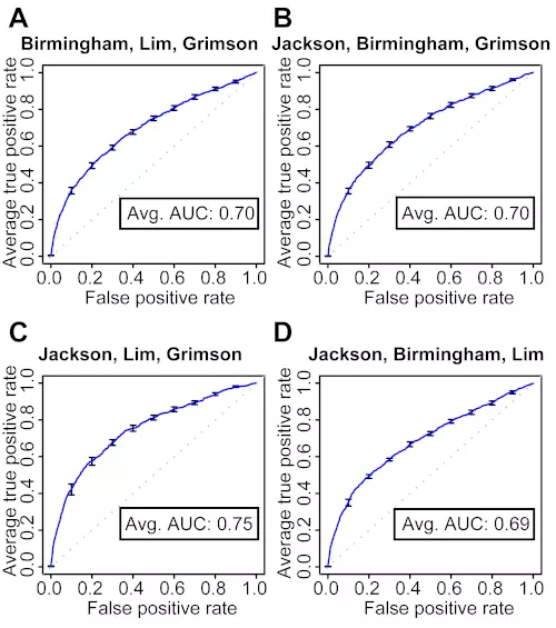
Figure S1. 10-fold cross-validation of target site level classifiers trained on three microarray datasets.
The ROC graphs show the classification performance of four classifiers trained with three microarray datasets at the target site level. The curve is the average ROC curve of the ten individual cross-validation test results; error bars show standard errors. Dotted lines illustrate random prediction. Avg. AUC is the average of the area under the curve (AUC; ROC score) of the ten individual cross-validation test results.
(A) Trained with the Birmingham, Lim and Grimson datasets.
(B) Trained with the Jackson, Birmingham and Grimson datasets.
(C) Trained with the Jackson, Lim and Grimson datasets.
(D) Trained with the Jackson, Birmingham and Lim datasets.
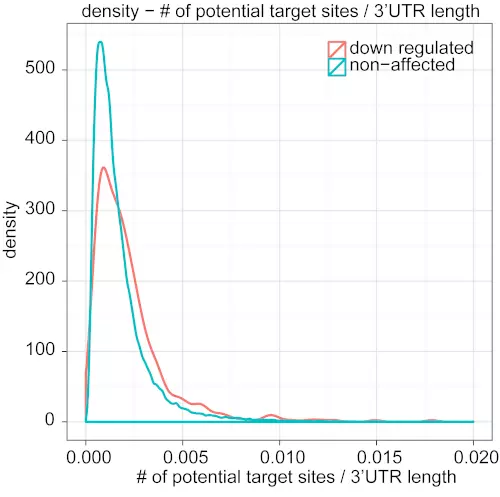
Figure S2. Density plot for the number of potential target sites divided by 3’UTR length.
It shows the density distribution of the values calculated by the number of miRNA potential sites divided by the 3’ UTR length. The red line indicates the distribution of down-regulated genes whereas the blue line is for the non-affected genes. The difference between two density distributions is very significant (Kolmogorov-Smirnov test, p-value: 3.862e-11).
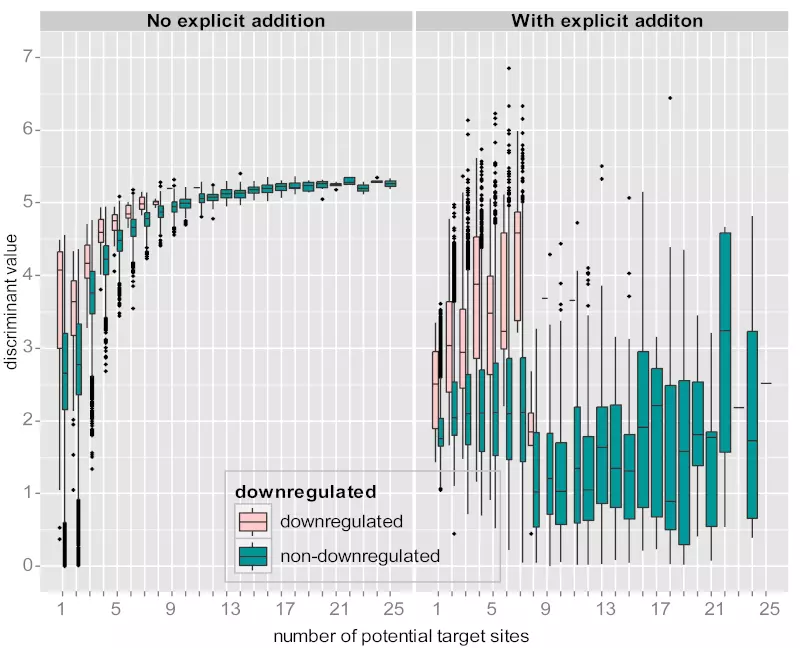
Figure S3. Comparison between two SVM trainings with or without explicit addition of negative records.
Two box plots show the number of potential target sites vs. discriminant values from mRNA level training. The left panel shows the distributions of discriminant values by the number of potential target sites for the classifier trained without any explicit additional of negative records. The right panel shows the classifier trained with data enriched with 1000 randomly selected non-target genes with more than 7 target sites. Records with the number of target sites >25 and/or negative discriminant values were disregarded. Whereas the left box plot shows that discriminant values for negative (non-downregulated) genes generally increase with increasing number of potential target sites, the right box plot indicates that the discriminant values for negative genes are relatively stable.
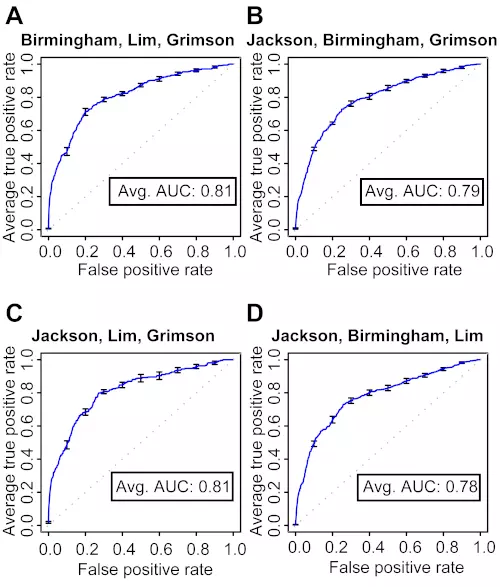
Figure S4. 10-fold cross-validation of mRNA level classifiers trained on three microarray datasets.
The ROC graphs show the classification performance of four classifiers trained with three different combinations of microarray datasets at the mRNA level. The curve is the average ROC curve of the ten individual cross-validation test results; error bars show standard errors. Dotted lines illustrate a random prediction. Avg. AUC is the average of the area under the curve (AUC; ROC score) of the ten individual cross-validation test results.
(A) Trained with the Birmingham, Lim and Grimson datasets.
(B) Trained with the Jackson, Birmingham and Grimson datasets.
(C) Trained with the Jackson, Lim and Grimson datasets.
(D) Trained with the Jackson, Birmingham and Lim datasets.
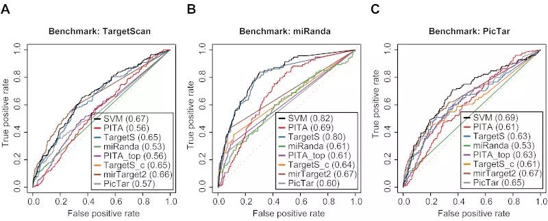
Figure S5. Three method-specific benchmarks of 8 different algorithms on the Linsley dataset.
Receiver operating characteristic (ROC) graphs show the performances of 8 different target prediction algorithms; SVM, PITA All (PITA), PITA Top (PITA_top), TargetScan (TargetS), TargetScan with conserved genes (TargetS_c), MicroCosm miRanda (miRanda), mirTarget2, and PicTar, on the Linsley dataset. Dotted lines illustrate random prediction. The values of the area under the ROC curve (AUC) are shown in the legend box. The benchmarks used for the evaluation were (A) ROC with TargetScan dataset, (B) ROC with miRanda dataset, and (C) ROC with PicTar dataset.
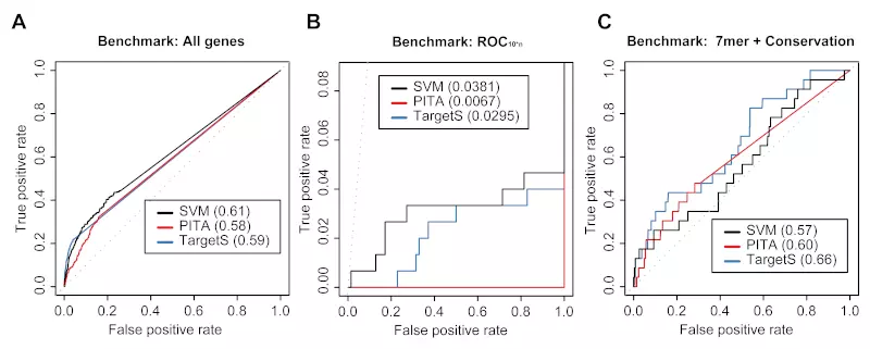
Figure S6. siRNA benchmarks on the Jackson dataset.
Receiver operating characteristic (ROC) graphs show the performance of 3 different target prediction algorithms – SVM not trained on Jackson dataset (SVM), PITA, and TargetScan (TargetS) – on the Jackson dataset. The SVM classifier was trained with the Lim, Birmingham and Grimson datasets. Dotted lines illustrate random prediction. The ROC scores are shown in the legend box. The benchmarks used for the evaluation were (A) ROC with All genes, (B) ROC10*n, and (C) ROC with 7mer + Conservation.
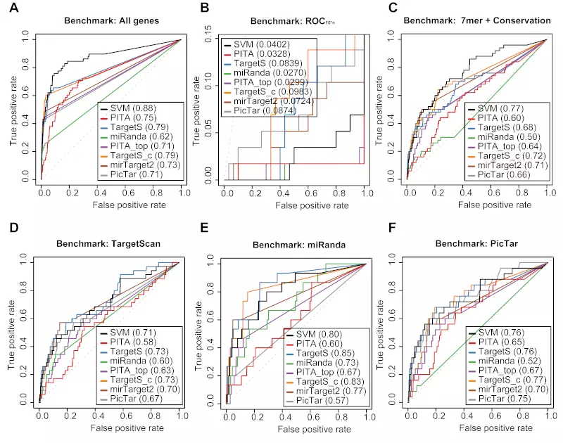
Figure S7. miRNA benchmarks on the Lim dataset.
Receiver operating characteristic (ROC) graphs show the performances of 8 different target prediction algorithms – SVM not trained on Lim dataset (SVM), PITA All (PITA), PITA Top (PITA_top), TargetScan (TargetS), TargetScan with conserved genes (TargetS_c), MicroCosm miRanda (miRanda), mirTarget2 and PicTar – on the Lim dataset. The SVM classifier was trained with the Jackon, Birmingham and Grimson datasets. Dotted lines illustrate random prediction. The values of the area under the ROC curve (AUC) are shown in the legend box. The benchmarks used for the evaluation were (A) ROC with TargetScan dataset, (B) ROC with miRanda dataset, (C) ROC with PicTar dataset, (D) ROC with TargetScan dataset, (E) ROC with miRanda dataset, and (F) ROC with PicTar dataset.
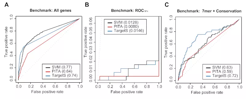
Figure S8. siRNA benchmarks on the Birmingham dataset.
Receiver operating characteristic (ROC) graphs show the performances of 3 different target prediction algorithms – SVM not trained on Birmingham dataset (SVM), PITA, and TargetScan (TargetS) – on the Birmingham dataset. The SVM classifier was trained with the Jackson, Lim and Grimon datasets. Dotted lines illustrate random prediction. The ROC scores are shown in the legend box. The benchmarks used for the evaluation were (A) ROC with All genes, (B) ROC10*n, and (C) ROC with 7mer + Conservation.
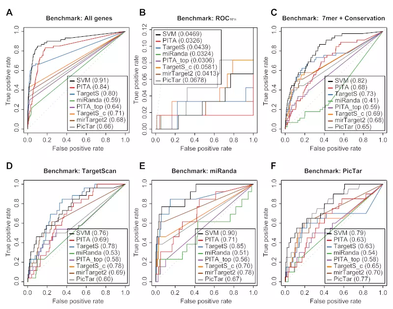
Figure S9. miRNA benchmarks on the Grimson dataset.
Receiver operating characteristic (ROC) graphs show the performances of 8 different target prediction algorithms – SVM not trained on Grimson dataset (SVM), PITA All (PITA), PITA Top (PITA_top), TargetScan (TargetS), TargetScan with conserved genes (TargetS_c), MicroCosm miRanda (miRanda), mirTarget2 and PicTar – on the Grimson dataset. The SVM classifier was trained with the Jackon, Lim, and Birmingham datasets. Dotted lines illustrate random prediction. The values of the area under the ROC curve (AUC) are shown in the legend box. The benchmarks used for the evaluation were (A) ROC with TargetScan dataset, (B) ROC with miRanda dataset, (C) ROC with PicTar dataset, (D) ROC with TargetScan dataset, (E) ROC with miRanda dataset, and (F) ROC with PicTar dataset.
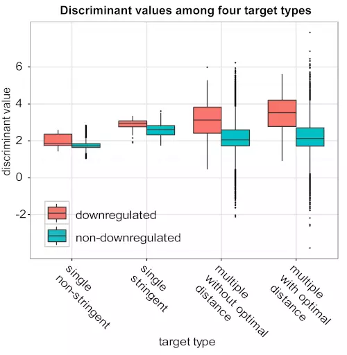
Figure S10. Targets with optimal distance sites show higher average discriminant value than other three target types.
The boxplot shows the comparison of mRNA level discriminant values among four different target types. The result shows our SVM approach gives scores as the preference: “multiple with optimal distance” > “multiple without optimal distance” > “single stringent” > “single non-stringent”.
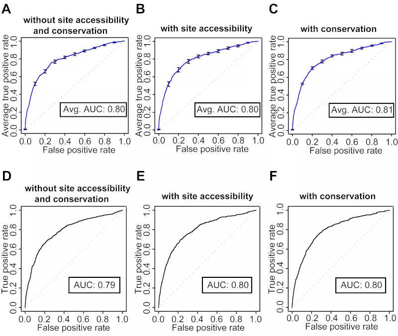
Figure S11. Adding site accessibility and sequence conservation features did not affect target prediction accuracy.
Receiver operating characteristic (ROC) graphs show the classification performance of three mRNA level classifiers. These classifiers had the same mRNA level features, but their discriminant values were generated by three different target site classifiers: (i) neither site accessibility nor sequence conservation used, (ii) with site accessibility and, (iii) with conservational information. Panels A-C show the three classifiers’ 10-fold cross-validation performance. The curve is the average ROC curve of the ten individual cross-validation test results; error bars show standard errors; Avg. AUC is the average of the area under the curve (AUC; ROC score) of the ten individual cross-validation test results. Panels D-F show the three classifiers’ performance on the independent (Linsley) dataset; ROC graphs were plotted by only considering the genes with prediction scores in the Linsley dataset. Dotted lines illustrate random prediction.
(A) 10-fold cross-validation of the classifier with neither site accessibility nor sequence conservation used
(B) 10-fold cross-validation of the classifier with site accessibility
(C) 10-fold cross-validation of the classifier with sequence conservation
(D) Classifier with neither site accessibility nor conservational information tested on the independent dataset
(E) Classifier with site accessibility tested on the independent dataset
(F) Classifier with sequence conservation tested on the independent dataset
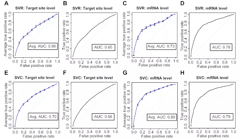
Figure S12. SVC performs better than SVR at both target site and mRNA levels.
The ROC graphs show the prediction performance of SVM regression (SVR) and SVM classification (SVC). Panels A, C, E, and G show the models’ 10-fold cross-validation performance. The curve is the average ROC curve of the ten individual cross-validation test results; error bars show standard errors; Avg. AUC is the average of the area under the curve (AUC; ROC score) of the ten individual cross-validation test results. Panels B, D, F, and H show the models’ performance on the independent (Linsley) dataset; ROC graphs were plotted by only considering the genes with SVC and SVR prediction scores in the Linsley dataset. Dotted lines illustrate random prediction. SVR and SVC show very similar performance, but SVC shows slightly better performance than SVR at both target site and mRNA levels.
(A) 10-fold cross-validation of SVR target site level
(B) Target site level SVR classifier tested on the independent dataset
(C) 10-fold cross-validation of SVR mRNA level
(D) mRNA level SVR classifier tested on the independent dataset
(E) 10-fold cross-validation of SVC target site level
(F) Target site level SVC classifier tested on the independent dataset
(G) 10-fold cross-validation of SVC mRNA level
(H) mRNA level SVC classifier tested on the independent dataset
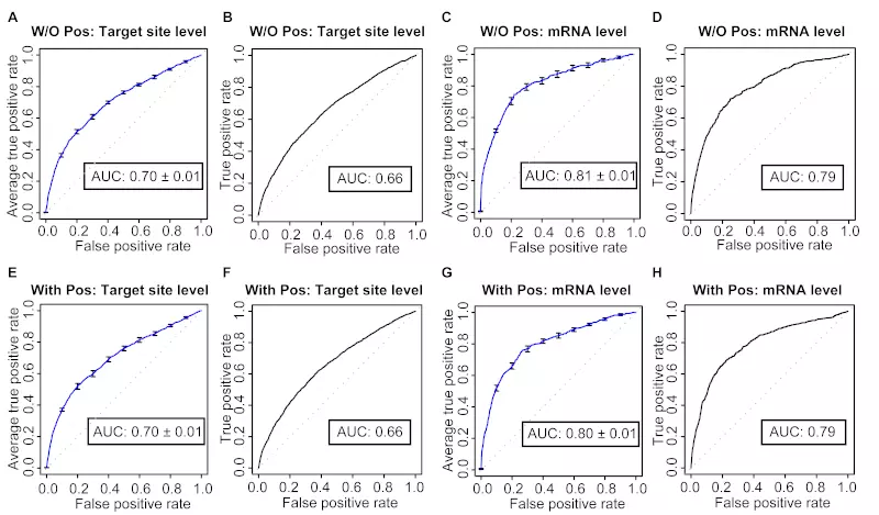
Figure S13. SVM performance is similar between the training set with up-regulated genes and the one without up-regulated genes.
The ROC graphs show the prediction performance of two SVM classifiers trained either with or without up-regulated genes. Panels A, C, E, and G show the models’ 10-fold cross-validation performance. The curve is the average ROC curve of the ten individual cross-validation test results; error bars show standard errors; Avg. AUC is the average of the area under the curve (AUC; ROC score) of the ten individual cross-validation test results. Panels B, D, F, and H show the models’ performance on the independent (Linsley) dataset; ROC graphs were plotted by only considering the genes with SVM prediction scores in the Linsley dataset. Dotted lines illustrate random prediction. Two classifiers show almost identical performances in terms of both ROC sores and ROC curves.
(A) 10-fold cross-validation of SVM without up-regulated genes at target site level
(B) Target site level SVM without up-regulated genes tested on the independent dataset
(C) 10-fold cross-validation of SVM without up-regulated genes at mRNA level
(D) mRNA level SVM without up-regulated genes tested on the independent dataset
(E) 10-fold cross-validation of SVM with up-regulated genes at target site level
(F) Target site level SVM with up-regulated genes tested on the independent dataset
(G) 10-fold cross-validation of SVM with up-regulated genes at mRNA level
(H) mRNA level SVM with up-regulated genes tested on the independent dataset
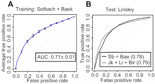
Figure S14. Two-step SVM retains the performance when trained with proteomics data.
(A) SVM classifier was trained by the Selbach and Baek datasets. The definitions of the error bars, AUC, true positive and false positive rates were the same as described in Figure 2. (B) Both proteomics and transcriptomics classifiers were tested on the Linsley dataset. Proteomics data contains the Selbach and Baek datasets, whereas Transcriptomics contains the Jackson, Lim, Birmingham, and Grimson datasets. The ROC scores were shown in the legend box.

Figure S15. Benchmarks on the Selbach dataset.
Receiver operating characteristic (ROC) graphs show the performances of 8 different target prediction algorithms – SVM, PITA All (PITA), PITA Top (PITA_top), TargetScan (TargetS), TargetScan with conserved genes (TargetS_c), MicroCosm miRanda (miRanda), mirTarget2 and PicTar – on the Selbach dataset. Dotted lines illustrate random prediction. The ROC scores are shown in the legend box. The benchmarks used for the evaluation were, (A) ROC with TargetScan dataset, (B) ROC with miRanda dataset, and (C) ROC with PicTar dataset.
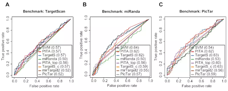
Figure S16. Benchmarks on the Baek dataset.
Receiver operating characteristic (ROC) graphs show the performances of 8 different target prediction algorithms – SVM, PITA All (PITA), PITA Top (PITA_top), TargetScan (TargetS), TargetScan with conserved genes (TargetS_c), MicroCosm miRanda (miRanda), mirTarget2 and PicTar – on the Baek dataset. Dotted lines illustrate random prediction. The ROC scores are shown in the legend box. The benchmarks used for the evaluation were (A) ROC with TargetScan dataset, (B) ROC with miRanda dataset, and (C) ROC with PicTar dataset.
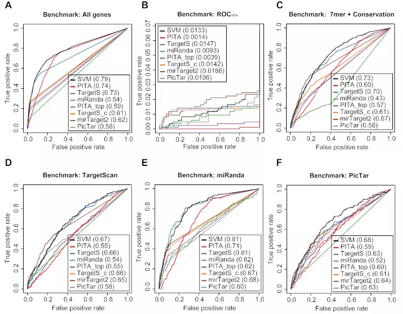
Figure S17. Benchmarks on the Linsley dataset with positive record threshold by log ratio -0.1.
Receiver operating characteristic (ROC) graphs show the performances of 8 different target prediction algorithms – SVM, PITA All (PITA), PITA Top (PITA_top), TargetScan (TargetS), TargetScan with conserved genes (TargetS_c), MicroCosm miRanda (miRanda), mirTarget2 and PicTar – on the Linsley dataset. Dotted lines illustrate random prediction. The ROC scores are shown in the legend box. Positive records (down-regulated) were selected by log ratio value -0.1 instead of the default value -0.2. The benchmarks used for the evaluation were (A) ROC with All genes, (B) ROC10*n, (C) ROC with 7mer + Conservation, (D) ROC with TargetScan dataset, (E) ROC with miRanda dataset, and (F) ROC with PicTar dataset.
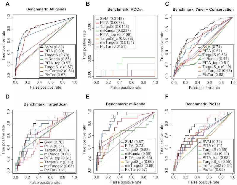
Figure S18. Benchmarks on the Linley dataset with positive record threshold by log ratio -0.3.
Receiver operating characteristic (ROC) graphs show the performances of 8 different target prediction algorithms – SVM, PITA All (PITA), PITA Top (PITA_top), TargetScan (TargetS), TargetScan with conserved genes (TargetS_c), MicroCosm miRanda (miRanda), mirTarget2 and PicTar – on the Linsley dataset. Dotted lines illustrate random prediction. The ROC scores are shown in the legend box. Positive records (down-regulated) were selected by log ratio value -0.3 instead of the default value -0.2. The benchmarks used for the evaluation were (A) ROC with All genes, (B) ROC10*n, (C) ROC with 7mer + Conservation, (D) ROC with TargetScan dataset, (E) ROC with miRanda dataset, and (F) ROC with PicTar dataset.
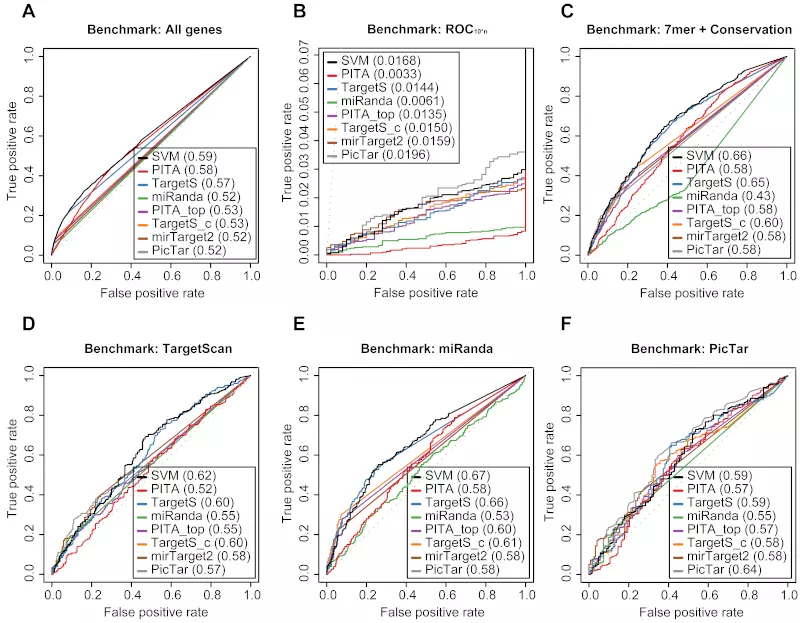
Figure S19. Benchmarks on the Selbach dataset with positive record threshold by log ratio -0.1.
Receiver operating characteristic (ROC) graphs show the performances of 8 different target prediction algorithms – SVM, PITA All (PITA), PITA Top (PITA_top), TargetScan (TargetS), TargetScan with conserved genes (TargetS_c), MicroCosm miRanda (miRanda), mirTarget2 and PicTar – on the Selbach dataset. Dotted lines illustrate random prediction. The ROC scores are shown in the legend box. Positive records (down-regulated) were selected by log ratio value -0.1 instead of the default value -0.2. The benchmarks used for the evaluation were (A) ROC with All genes, (B) ROC10*n, (C) ROC with 7mer + Conservation, (D) ROC with TargetScan dataset, (E) ROC with miRanda dataset, and (F) ROC with PicTar dataset.
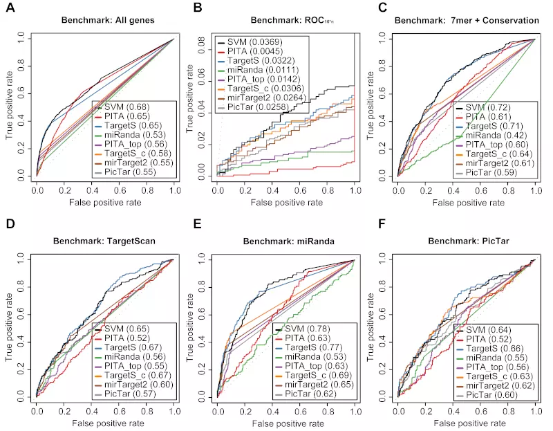
Figure S20. Benchmarks on the Selbach dataset with positive record threshold by log ratio -0.3.
Receiver operating characteristic (ROC) graphs show the performances of 8 different target prediction algorithms – SVM, PITA All (PITA), PITA Top (PITA_top), TargetScan (TargetS), TargetScan with conserved genes (TargetS_c), MicroCosm miRanda (miRanda), mirTarget2 and PicTar – on the Selbach dataset. Dotted lines illustrate random prediction. The ROC scores are shown in the legend box. Positive records (down-regulated) were selected by log ratio value -0.3 instead of the default value -0.2. The benchmarks used for the evaluation were (A) ROC with All genes, (B) ROC10*n, (C) ROC with 7mer + Conservation, (D) ROC with TargetScan dataset, (E) ROC with miRanda dataset, and (F) ROC with PicTar dataset.
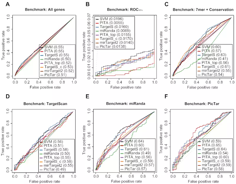
Figure S21. Benchmarks on the Baek dataset with positive record threshold by log ratio -0.1.
Receiver operating characteristic (ROC) graphs show the performances of 8 different target prediction algorithms – SVM, PITA All (PITA), PITA Top (PITA_top), TargetScan (TargetS), TargetScan with conserved genes (TargetS_c), MicroCosm miRanda (miRanda), mirTarget2 and PicTar – on the Baek dataset. Dotted lines illustrate random prediction. The ROC scores are shown in the legend box. Positive records (down-regulated) were selected by log ratio value -0.1 instead of the default value -0.2. The benchmarks used for the evaluation were (A) ROC with All genes, (B) ROC10*n, (C) ROC with 7mer + Conservation, (D) ROC with TargetScan dataset, (E) ROC with miRanda dataset, and (F) ROC with PicTar dataset.
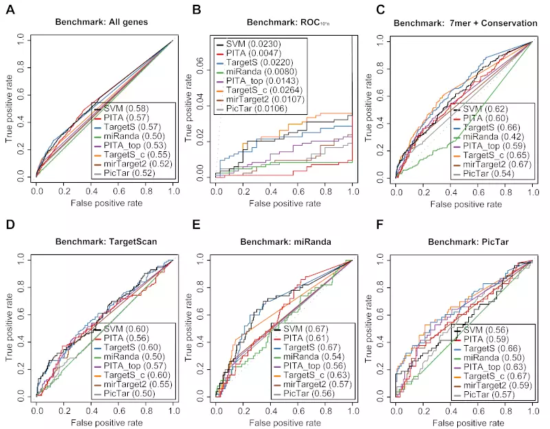
Figure S22. Benchmarks on the Baek dataset with positive record threshold by log ratio -0.3.
Receiver operating characteristic (ROC) graphs show the performances of 8 different target prediction algorithms – SVM, PITA All (PITA), PITA Top (PITA_top), TargetScan (TargetS), TargetScan with conserved genes (TargetS_c), MicroCosm miRanda (miRanda), mirTarget2 and PicTar – on the Baek dataset. Dotted lines illustrate random prediction. The ROC scores are shown in the legend box. Positive records (down-regulated) were selected by log ratio value -0.3 instead of the default value -0.2. The benchmarks used for the evaluation were (A) ROC with All genes, (B) ROC10*n, (C) ROC with 7mer + Conservation, (D) ROC with TargetScan dataset, (E) ROC with miRanda dataset, and (F) ROC with PicTar dataset.
References
- Birmingham A, Anderson EM, Reynolds A, Ilsley-Tyree D, Leake D, Fedorov Y, et al. 3′ UTR seed matches, but not overall identity, are associated with RNAi off-targets. Nature Methods 2006;3:199–204. https://doi.org/10.1038/nmeth854.
- Linsley PS, Schelter J, Burchard J, Kibukawa M, Martin MM, Bartz SR, et al. Transcripts targeted by the MicroRNA-16 family cooperatively regulate cell cycle progression. Molecular and Cellular Biology 2007;27:2240–52. https://doi.org/10.1128/mcb.02005-06.
- Gribskov M, Robinson NL. Use of receiver operating characteristic (ROC) analysis to evaluate sequence matching. Computers & Chemistry 1996;20:25–33. https://doi.org/10.1016/s0097-8485(96)80004-0.
- Gaidatzis D, Nimwegen E van, Hausser J, Zavolan M. Inference of miRNA targets using evolutionary conservation and pathway analysis. BMC Bioinformatics 2007;8:69. https://doi.org/10.1186/1471-2105-8-69.
- Grimson A, Farh KK-H, Johnston WK, Garrett-Engele P, Lim LP, Bartel DP. MicroRNA targeting specificity in mammals: determinants beyond seed pairing. Molecular Cell 2007;27:91–105. https://doi.org/10.1016/j.molcel.2007.06.017.
- Hammell M, Long D, Zhang L, Lee A, Carmack CS, Han M, et al. mirWIP: microRNA target prediction based on microRNA-containing ribonucleoprotein-enriched transcripts. Nature Methods 2008;5:813–9. https://doi.org/10.1038/nmeth.1247.
- Jackson AL, Burchard J, Schelter J, Chau BN, Cleary M, Lim L, et al. Widespread siRNA "off-target" transcript silencing mediated by seed region sequence complementarity. RNA 2006;12:1179–87. https://doi.org/10.1261/rna.25706.
- Lim LP, Lau NC, Garrett-Engele P, Grimson A, Schelter JM, Castle J, et al. Microarray analysis shows that some microRNAs downregulate large numbers of target mRNAs. Nature 2005;433:769–73. https://doi.org/10.1038/nature03315.
- Huang JC, Babak T, Corson TW, Chua G, Khan S, Gallie BL, et al. Using expression profiling data to identify human microRNA targets. Nature Methods 2007;4:1045–9. https://doi.org/10.1038/nmeth1130.
- Sales G, Coppe A, Bicciato S, Bortoluzzi S, Romualdi C. Impact of probe annotation on the integration of miRNA-mRNA expression profiles for miRNA target detection. Nucleic Acids Research 2010;38:e97–e97. https://doi.org/10.1093/nar/gkp1239.
- Kertesz M, Iovino N, Unnerstall U, Gaul U, Segal E. The role of site accessibility in microRNA target recognition. Nature Genetics 2007;39:1278–84. https://doi.org/10.1038/ng2135.
- Long D, Lee R, Williams P, Chan CY, Ambros V, Ding Y. Potent effect of target structure on microRNA function. Nature Structural & Molecular Biology 2007;14:287–94. https://doi.org/10.1038/nsmb1226.
- Baek D, Villén J, Shin C, Camargo FD, Gygi SP, Bartel DP. The impact of microRNAs on protein output. Nature 2008;455:64–71. https://doi.org/10.1038/nature07242.
- Sethupathy P, Megraw M, Hatzigeorgiou AG. A guide through present computational approaches for the identification of mammalian microRNA targets. Nature Methods 2006;3:881–6. https://doi.org/10.1038/nmeth954.
- Enright AJ, John B, Gaul U, Tuschl T, Sander C, Marks DS. MicroRNA targets in Drosophila. Genome Biology 2003;5:R1. https://doi.org/10.1186/gb-2003-5-1-r1.